The Illusory Divide, the Hidden Unity: RNNs and ODEs — An Introduction to "Fancy" RNNs
I had already made up my mind to stop playing with RNNs, but last week, while thinking things over, I suddenly realized that RNNs actually correspond to numerical solvers for ODEs (ordinary differential equations). This gave me a concrete idea for something I'd long wanted to do — use deep learning to tackle some pure mathematics problems. This turns out to be a rather interesting and useful result, so let me walk through it. Incidentally, this post also involves writing custom RNNs by hand, so it can also serve as a simple tutorial on building your own custom RNN layer.
Note: this post is not an introduction to the recently popular "Neural ODE" (though there is some connection).
RNN Basics
What is an RNN?
As everyone knows, RNN stands for "Recurrent Neural Network." Unlike CNNs, "RNN" is really a blanket term for a whole family of models, not a single model. Simply put, given an input vector sequence $(\boldsymbol{x}_1,\boldsymbol{x}_2,\dots,\boldsymbol{x}_T)$ and an output vector sequence $(\boldsymbol{y}_1,\boldsymbol{y}_2,\dots,\boldsymbol{y}_T)$, any model satisfying the recursive relation
$$\boldsymbol{y}_t=f(\boldsymbol{y}_{t-1}, \boldsymbol{x}_t, t)\tag{1}$$
can be called an RNN. That's precisely why the original vanilla RNN, along with improved variants such as GRU, LSTM, SRU, and so on, are all called RNNs — they're all special cases of the equation above. There are even things that don't look related to RNNs at all on the surface, such as the computation of the denominator in CRF that I introduced not long ago — that too is actually just a simple RNN.
In plain terms, RNN is really just recursive computation. more
Writing Your Own RNN
Let's first look at how to write a custom RNN quickly and easily in Keras.
In fact, whether in Keras or in raw TensorFlow, building your own custom RNN isn't all that complicated. In Keras, you just need to write the per-step recursive function; in TensorFlow it's a bit more involved, since you need to wrap the per-step recursive function into an RNNCell class. Below I'll show how to implement the most basic RNN using Keras:
$$\boldsymbol{y}_t=\tanh(\boldsymbol{W}_1 \boldsymbol{y}_{t-1} + \boldsymbol{W}_2 \boldsymbol{x}_t + \boldsymbol{b})\tag{2}$$
The code is very simple:
#! -*- coding: utf-8- -*-

from keras.layers import Layer
import keras.backend as K

class My_RNN(Layer):

    def __init__(self, output_dim, **kwargs):
        self.output_dim = output_dim # 输出维度
        super(My_RNN, self).__init__(**kwargs)

    def build(self, input_shape): # 定义可训练参数
        self.kernel1 = self.add_weight(name='kernel1',
                                      shape=(self.output_dim, self.output_dim),
                                      initializer='glorot_normal',
                                      trainable=True)
        self.kernel2 = self.add_weight(name='kernel2',
                                      shape=(input_shape[-1], self.output_dim),
                                      initializer='glorot_normal',
                                      trainable=True)
        self.bias = self.add_weight(name='bias',
                                      shape=(self.output_dim,),
                                      initializer='glorot_normal',
                                      trainable=True)

    def step_do(self, step_in, states): # 定义每一步的迭代
        step_out = K.tanh(K.dot(states[0], self.kernel1) +
                          K.dot(step_in, self.kernel2) +
                          self.bias)
        return step_out, [step_out]

    def call(self, inputs): # 定义正式执行的函数
        init_states = [K.zeros((K.shape(inputs)[0],
                                self.output_dim)
                              )] # 定义初始态(全零)
        outputs = K.rnn(self.step_do, inputs, init_states) # 循环执行step_do函数
        return outputs[0] # outputs是一个tuple,outputs[0]为最后时刻的输出,
                          # outputs[1]为整个输出的时间序列,output[2]是一个list,
                          # 是中间的隐藏状态。

    def compute_output_shape(self, input_shape):
        return (input_shape[0], self.output_dim)
As you can see, although there are quite a few lines of code, most of them are just boilerplate. What actually defines the RNN is the function step_do, which takes two inputs: step_in and states. Here step_in is a tensor of shape (batch_size, input_dim), representing the sample at the current time step $\boldsymbol{x}_t$, and states is a list representing $\boldsymbol{y}_{t-1}$ along with some intermediate variables. It's especially important to note that states is a list of tensors, not a single tensor — this is because during the recursion we may need to carry several intermediate variables at once, not just $\boldsymbol{y}_{t-1}$; for instance, LSTM needs two state tensors. Finally, step_do must return $\boldsymbol{y}_t$ and the new states — this is the calling convention that a step_do function must follow.
As for the function K.rnn, it takes three basic arguments (there are others too — check the official documentation for those). The first argument is the step_do function we just wrote, the second is the input time series, and the third is the initial state, consistent with the states mentioned above — so naturally init_states is also a list of tensors, which by default we initialize to all zeros.
ODE Basics
What is an ODE?
ODE stands for "Ordinary Differential Equation." Here we mean a general system of ordinary differential equations:
$$\dot{\boldsymbol{x}}(t)=\boldsymbol{f}\big(\boldsymbol{x}(t), t\big)\tag{3}$$
The field that studies ODEs is often directly called "dynamics" or "dynamical systems," since Newtonian mechanics is, in essence, nothing more than a system of ODEs.
ODEs can produce an extraordinarily rich variety of functions. For example, $e^t$ is in fact the solution to $\dot{x}=x$, and both $\sin t$ and $\cos t$ are solutions to $\ddot{x}+x=0$ (with different initial conditions). Indeed, I recall that some textbooks define the $e^t$ function directly via the differential equation $\dot{x}=x$. Beyond these elementary functions, many special functions that we can name but don't really understand — hypergeometric functions, Legendre functions, Bessel functions, and so on — are all derived via ODEs.
In short, ODEs can produce, and have already produced, all manner of exotic functions.
Solving ODEs Numerically
ODEs with exact closed-form solutions are actually quite rare, so numerical methods are needed most of the time.
Numerical solution of ODEs is already a very mature discipline, and I won't go into much detail here — I'll just introduce the most basic iterative formula, due to Euler:
$$\boldsymbol{x}(t + h) = \boldsymbol{x}(t) + h \boldsymbol{f}\big(\boldsymbol{x}(t), t\big)\tag{4}$$
Here $h$ is the step size. The origin of Euler's method is simple: it approximates the derivative term $\dot{\boldsymbol{x}}(t)$ using
$$\frac{\boldsymbol{x}(t + h) - \boldsymbol{x}(t)}{h}\tag{5}$$
Given an initial condition $\boldsymbol{x}(0)$, we can then use $(4)$ to iteratively compute the result at each time point, step by step.
ODE and RNN
An ODE is Also an RNN
Compare $(4)$ and $(1)$ carefully — do you notice any connection?
In $(1)$, $t$ is an integer variable, whereas in $(4)$, $t$ is a floating-point variable. Apart from that, there's no obvious difference between $(4)$ and $(1)$. In fact, in $(4)$ we can take $h$ as the unit of time and write $t=nh$, so that $(4)$ becomes
$$\boldsymbol{x}\big((n+1)h\big) = \boldsymbol{x}(nh) + h \boldsymbol{f}\big(\boldsymbol{x}(nh), nh\big)\tag{6}$$
Now we can see that the time variable $n$ in $(6)$ is also an integer.
This tells us that: Euler's method for solving ODEs, $(4)$, is in fact nothing more than a special case of an RNN. This gives us some indirect insight into why RNNs are so powerful at fitting functions (especially for time-series data): we've seen that ODEs can produce a great many complex functions, and ODEs are merely a special case of RNNs — so RNNs can produce even more complex functions still.
Using RNNs to Solve ODEs
So we can write an RNN to solve an ODE — for example, take the example from A Competition Model Between Two Biological Populations:
$$\left\{\begin{aligned}\frac{dx_1}{dt}=r_1 x_1\left(1-\frac{x_1}{N_1}\right)-a_1 x_1 x_2 \\ \frac{dx_2}{dt}=r_2 x_2\left(1-\frac{x_2}{N_2}\right)-a_2 x_1 x_2\end{aligned}\right.\tag{7}$$
We can write:
#! -*- coding: utf-8- -*-

from keras.layers import Layer
import keras.backend as K

class ODE_RNN(Layer):

    def __init__(self, steps, h, **kwargs):
        self.steps = steps
        self.h = h
        super(ODE_RNN, self).__init__(**kwargs)

    def step_do(self, step_in, states): # 定义每一步的迭代
        x = states[0]
        r1,r2,a1,a2,iN1,iN2 = 0.1,0.3,0.0001,0.0002,0.002,0.003
        _1 = r1 * x[:,0] * (1 - iN1 * x[:,0]) - a1 * x[:,0] * x[:,1]
        _2 = r2 * x[:,1] * (1 - iN2 * x[:,1]) - a2 * x[:,0] * x[:,1]
        _1 = K.expand_dims(_1, 1)
        _2 = K.expand_dims(_2, 1)
        _ = K.concatenate([_1, _2], 1)
        step_out = x + self.h * _
        return step_out, [step_out]

    def call(self, inputs): # 这里的inputs就是初始条件
        init_states = [inputs]
        zeros = K.zeros((K.shape(inputs)[0],
                         self.steps,
                         K.shape(inputs)[1])) # 迭代过程用不着外部输入,所以
                                              # 指定一个全零输入,只为形式上的传入
        outputs = K.rnn(self.step_do, zeros, init_states) # 循环执行step_do函数
        return outputs[1] # 这次我们输出整个结果序列

    def compute_output_shape(self, input_shape):
        return (input_shape[0], self.steps, input_shape[1])

from keras.models import Sequential
import numpy as np
import matplotlib.pyplot as plt

steps,h = 1000,0.1

M = Sequential()
M.add(ODE_RNN(steps, h, input_shape=(2,)))
M.summary()

# 直接前向传播就输出解了
result = M.predict(np.array([[100, 150]]))[0] # 以[100, 150]为初始条件进行演算
times = np.arange(1, steps+1) * h

# 绘图
plt.plot(times, result[:,0])
plt.plot(times, result[:,1])
plt.savefig('test.png')
The whole process is easy to follow, though two points deserve mention. First, since the system of equations $(7)$ is only two-dimensional and doesn't lend itself easily to matrix operations, in step_do I operate directly component-wise (the x[:,0], x[:,1] in the code); if the equations are higher-dimensional and can be written as matrix operations, it would be more efficient to do so directly. Second, notice that once the model is fully assembled, calling predict directly gives us the result — no "training" is needed.
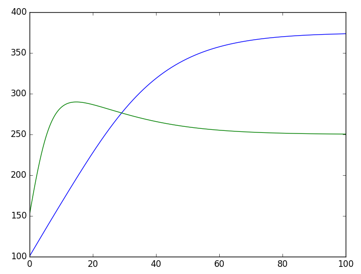 RNN solving the two-species competition model
Inferring ODE Parameters
The previous section shows that the forward pass of an RNN corresponds to Euler's method for solving an ODE — so what does backpropagation correspond to?
In practical problems, there's a class of problems called "model inference," where, given observed experimental data, one tries to guess the underlying model that the data conforms to (mechanistic inference). This kind of problem is generally tackled in two steps: first, guess the form of the model; second, determine the model's parameters. Suppose the data can be described by an ODE, and suppose we already know the form of this ODE — then we need to estimate its parameters.
If the ODE could be solved exactly in closed form, this would just be a very simple regression problem. But as noted earlier, most ODEs have no closed-form solution, so numerical methods are essential. This is exactly what backpropagation through the RNN corresponding to the ODE accomplishes: the forward pass solves the ODE (the RNN's prediction process), and naturally the backward pass infers the ODE's parameters (the RNN's training process). Here's a delightful fact: parameter inference for ODEs is a topic that has been studied extensively and rigorously, yet in deep learning it is merely one of the most basic applications of RNNs.
Let's save the solution data from the differential equation in the example above, then keep only a few points, and see whether we can recover the original differential equation. The solution data is:
$$\begin{array}{c|ccccccc} \hline \text{time} & 0 & 10 & 15 & 30 & 36 & 40 & 42\\ \hline x_1 & 100 & 165 & 197 & 280 & 305 & 318 & 324\\ \hline x_2 & 150 & 283 & 290 & 276 & 269 & 266 & 264\\ \hline \end{array}$$
Suppose we only know this finite set of data points, and we assume the form of equation $(7)$ is known — we then want to solve for its parameters. Let's modify the earlier code slightly:
#! -*- coding: utf-8- -*-

from keras.layers import Layer
import keras.backend as K

def my_init(shape, dtype=None): # 需要定义好初始化,这相当于需要实验估计参数的量级
    return K.variable([0.1, 0.1, 0.001, 0.001, 0.001, 0.001])

class ODE_RNN(Layer):

    def __init__(self, steps, h, **kwargs):
        self.steps = steps
        self.h = h
        super(ODE_RNN, self).__init__(**kwargs)

    def build(self, input_shape): # 将原来的参数设为可训练的参数
        self.kernel = self.add_weight(name='kernel',
                                      shape=(6,),
                                      initializer=my_init,
                                      trainable=True)
    def step_do(self, step_in, states): # 定义每一步的迭代
        x = states[0]
        r1,r2,a1,a2,iN1,iN2 = (self.kernel[0], self.kernel[1],
                               self.kernel[2], self.kernel[3],
                               self.kernel[4], self.kernel[5])
        _1 = r1 * x[:,0] * (1 - iN1 * x[:,0]) - a1 * x[:,0] * x[:,1]
        _2 = r2 * x[:,1] * (1 - iN2 * x[:,1]) - a2 * x[:,0] * x[:,1]
        _1 = K.expand_dims(_1, 1)
        _2 = K.expand_dims(_2, 1)
        _ = K.concatenate([_1, _2], 1)
        step_out = x + self.h * K.clip(_, -1e5, 1e5) # 防止梯度爆炸
        return step_out, [step_out]

    def call(self, inputs): # 这里的inputs就是初始条件
        init_states = [inputs]
        zeros = K.zeros((K.shape(inputs)[0],
                         self.steps,
                         K.shape(inputs)[1])) # 迭代过程用不着外部输入,所以
                                              # 指定一个全零输入,只为形式上的传入
        outputs = K.rnn(self.step_do, zeros, init_states) # 循环执行step_do函数
        return outputs[1] # 这次我们输出整个结果序列

    def compute_output_shape(self, input_shape):
        return (input_shape[0], self.steps, input_shape[1])

from keras.models import Sequential
from keras.optimizers import Adam
import numpy as np
import matplotlib.pyplot as plt

steps,h = 50, 1 # 用大步长,减少步数,削弱长时依赖,也加快推断速度
series = {0: [100, 150],
          10: [165, 283],
          15: [197, 290],
          30: [280, 276],
          36: [305, 269],
          40: [318, 266],
          42: [324, 264]}

M = Sequential()
M.add(ODE_RNN(steps, h, input_shape=(2,)))
M.summary()

# 构建训练样本
# 其实就只有一个样本序列,X为初始条件,Y为后续时间序列
X = np.array([series[0]])
Y = np.zeros((1, steps, 2))

for i,j in series.items():
    if i != 0:
        Y[0, int(i/h)-1] += series[i]

# 自定义loss
# 在训练的时候,只考虑有数据的几个时刻,没有数据的时刻被忽略
def ode_loss(y_true, y_pred):
    T = K.sum(K.abs(y_true), 2, keepdims=True)
    T = K.cast(K.greater(T, 1e-3), 'float32')
    return K.sum(T * K.square(y_true - y_pred), [1, 2])

M.compile(loss=ode_loss,
          optimizer=Adam(1e-4))

M.fit(X, Y, epochs=10000) # 用低学习率训练足够多轮

# 用训练出来的模型重新预测,绘图,比较结果
result = M.predict(np.array([[100, 150]]))[0]
times = np.arange(1, steps+1) * h

plt.clf()
plt.plot(times, result[:,0], color='blue')
plt.plot(times, result[:,1], color='green')
plt.plot(series.keys(), [i[0] for i in series.values()], 'o', color='blue')
plt.plot(series.keys(), [i[1] for i in series.values()], 'o', color='green')
plt.savefig('test.png')
The result can be seen in the following figure:
 Effect of using an RNN for ODE parameter estimation (scatter: limited experimental data, curve: estimated model)
The result is clearly satisfying.
Once Again, a Summary
This post introduced the RNN model in a general framework, along with how to write custom RNNs in Keras, and then revealed the connection between ODEs and RNNs. Building on this, it introduced the basic ideas behind using RNNs to solve ODEs directly, and using RNNs to infer ODE parameters. One reminder for readers: in backpropagation through RNN models, you need to be careful with initialization and gradient clipping, and choose the learning rate carefully, to prevent gradient explosion (gradient vanishing is just a matter of suboptimal optimization, but gradient explosion causes an outright crash — solving the gradient explosion problem is especially important).
In short, vanishing and exploding gradients are a classic pain point in RNNs. In fact, the fundamental reason for introducing models like LSTM and GRU was to solve the vanishing gradient problem in RNNs, while exploding gradients are typically dealt with by using tanh or sigmoid activation functions. But if we're using an RNN to solve an ODE, we don't get to choose the activation function freely (the activation function is part of the ODE itself), so we have no choice but to be careful with initialization and other measures. It's said that as long as initialization is done carefully, even using relu as the activation function in a plain RNN causes no trouble.
Translated automatically with claude-sonnet-5; all equations are reproduced verbatim from the source. Copyright remains with the original author.