A Two-Species Competition Model: LaTeX + Python

两生物种群竞争模型：LaTeX+Python 苏剑林 · 2014-12-15 · Biology differential equation analysis modeling qualitative

Foreword: This post is an assignment from my mathematical modeling course, exploring the properties of the solutions to a system of ordinary differential equations modeling competition between two biological populations, and demonstrating the basic ideas of the qualitative theory of differential equations. Of course, the most important purpose of this post is to showcase the perfect combination of LaTeX and Python. (All the figures in this post were generated with Python's Matplotlib module, while the document itself was typeset in LaTeX.)

Problem Statement

We study the competitive relationship between two populations living in the same natural environment. Suppose that when each population lives alone in this environment, its numbers evolve according to the Logistic law; and suppose further that when the two populations compete with each other, each slows down the growth rate of the other, with the reduction in growth rate proportional to the product of their population sizes. Under these assumptions, the ordinary differential equation model we obtain is

$$\begin{equation}\label{eq:jingzhengfangcheng}\left\{\begin{aligned}\frac{dx_1}{dt}=r_1 x_1\left(1-\frac{x_1}{N_1}\right)-a_1 x_1 x_2 \\ \frac{dx_2}{dt}=r_2 x_2\left(1-\frac{x_2}{N_2}\right)-a_2 x_1 x_2\end{aligned}\right.\end{equation}$$

In this post we analyze the properties of this equation from both a quantitative and a qualitative point of view. more

Model Analysis

Throughout the analysis, we use the following model parameters:

$$\begin{equation}\label{eq:fangchengcanshu}\left\{\begin{aligned} &r_1 = 0.1,\frac{1}{N_1}=0.002,a_1=0.0001\\ &r_2=0.3,\frac{1}{N_2}=0.003,a_2=0.0002\\ &x_1(0)=100,x_2(0)=150 \end{aligned}\right.\end{equation}$$

These parameters indicate that $x_1$ is a species with relatively slow growth, but with weaker intraspecific competition, and one that is not easily affected by species $x_2$; therefore, in the long run, species $x_1$ will dominate this natural environment. In contrast, species $x_2$ grows faster, but suffers from stronger intraspecific competition and is more easily affected by species $x_1$; hence, in the long-term competition, species $x_2$ will end up in a somewhat weaker position. The numerical solution below supports this conjecture.

Numerical solution

Combining $(1)$ and $(2)$, we solved this model numerically using Python. The result is shown in the figure below.

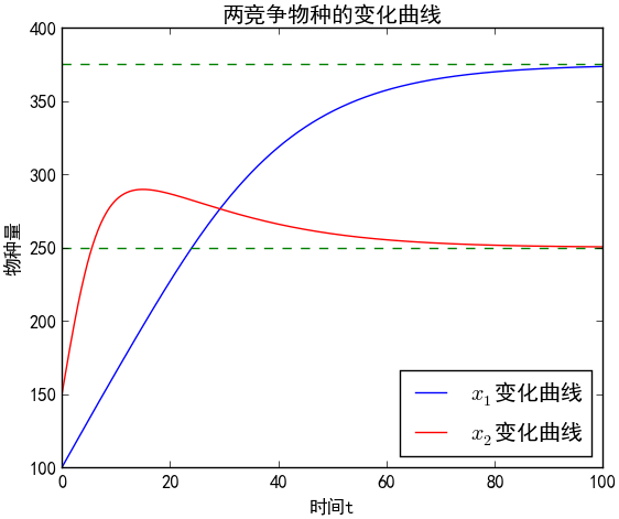Numerical solution of the competition model

The numerical solution shows that species $x_2$ initially grows quickly, reaches a maximum, then declines slowly and eventually stabilizes at 250, while species $x_1$ maintains a comparatively slower growth rate until it settles at the equilibrium value of 375. Next we analyze the properties of the equilibrium points of equation $(1)$.

Equilibrium points

The equation determining the equilibrium points of equation $(1)$ is

$$\begin{equation}\label{eq:pinghengdianfangcheng}\left\{\begin{aligned}r_1 x_1\left(1-\frac{x_1}{N_1}\right)-a_1 x_1 x_2=0 \\ r_2 x_2\left(1-\frac{x_2}{N_2}\right)-a_2 x_1 x_2=0\end{aligned}\right.\end{equation}$$

This equation has 4 solutions:

$$\begin{equation}\label{eq:pinghengdian} \left\{\begin{aligned}&x_1 =0\\&x_2 =0\end{aligned}\right., \quad \left\{\begin{aligned}&x_1 =0\\&x_2 =N_2\end{aligned}\right.,\quad \left\{\begin{aligned}&x_1 = N_1\\&x_2 =0\end{aligned}\right.,\quad \left\{\begin{aligned}&x_1 = \frac{N_1 r_2 (a_1 N_2 -r_1 )}{a_1 a_2 N_1 N_2-r_1 r_2}\\&x_2 =\frac{N_2 r_1 (a_2 N_1- r_2)}{a_1 a_2 N_1 N_2-r_1 r_2} \end{aligned}\right.\end{equation}$$

The first three equilibrium points are trivial, while the last one is non-trivial. We can observe that, with the given parameters $(2)$, equation $(1)$ eventually converges to the fourth equilibrium point, which indicates that this fourth equilibrium point has strong stability. Below, we analyze the stability of the equilibrium points and the global behavior of the equation using direction field and phase portrait diagrams.

Direction field

The figure below shows the direction field with respect to $(1)$ and $(2)$, in which the equilibrium points are marked with green dots. The shade of the arrow colors represents the speed of change at that point.

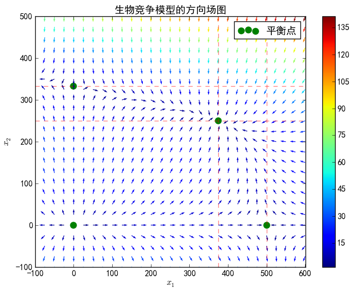Direction field of the competition model

From the direction field, the stability of the four equilibrium points can be determined fairly easily.

The first equilibrium point, at the bottom left, $(0,0)$, corresponds to the case where both populations are zero. It is an unstable equilibrium point: all the arrows point away from it, meaning that any small perturbation near this point will eventually drive the system away from it. In other words, as long as there is even a tiny amount of either species present, it will eventually grow and the system will settle into another equilibrium.
The second equilibrium point, at the top left, $(0,N_2)$, corresponds to the case where only species $x_2$ is present. It is an unstable equilibrium point (a saddle point): only the arrows on the vertical line through this point point toward it, while all other arrows point away from it. This shows that this equilibrium is somewhat more stable than $(0,0)$, but is still unstable — as long as a small amount of species $x_1$ is present, competition will drive the system away from the current equilibrium.
The third equilibrium point, at the bottom right, $(N_1,0)$, corresponds to the case where only species $x_1$ is present. It is likewise an unstable equilibrium point (a saddle point): only the arrows on the horizontal line through this point point toward it, while all other arrows point away from it. This shows that this equilibrium is somewhat more stable than $(0,0)$, but is still unstable — as long as a small amount of species $x_2$ is present, competition will drive the system away from the current equilibrium.
The fourth equilibrium point, at the top right, $\left(\frac{N_1 r_2 (a_1 N_2 -r_1 )}{a_1 a_2 N_1 N_2-r_1 r_2},\frac{N_2 r_1 (a_2 N_1- r_2)}{a_1 a_2 N_1 N_2-r_1 r_2}\right)$, corresponds to the case where both species coexist in balance. It is a stable equilibrium point: all the arrows near this point point toward it, meaning that even if the system deviates from this equilibrium, it will eventually return to it.

Phase trajectories

From the family of phase trajectories shown below, we can see the flow near the equilibrium points more clearly. Nearly all the trajectories within the first quadrant (the region corresponding to physically meaningful solutions) converge toward the fourth equilibrium point, which shows that this equilibrium has very strong stability — it is the final stable state for essentially any initial condition.

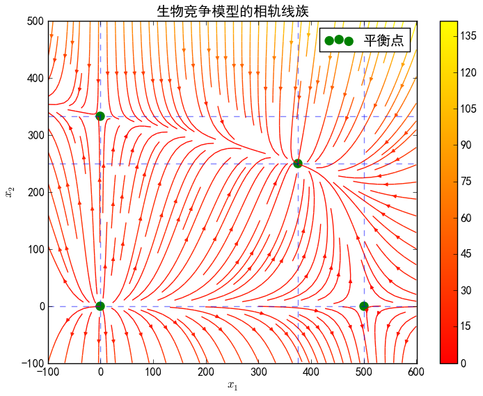Phase portrait of the competition model

We can observe that there are no closed orbits in the family of phase trajectories, which means the equation has no periodic oscillatory solutions.

Code Listing

The following code requires a Python 3 + NumPy + SciPy + Matplotlib environment.

Numerical solution

from scipy.integrate import odeint
import numpy as np
from scipy.optimize import leastsq
import matplotlib.pyplot as plt
plt.rcParams['font.sans-serif'] = ['SimHei'] #这两句用来正常显示中文标签
plt.rcParams['axes.unicode_minus'] = False

t = np.arange(0,100,0.1)

def deriv(w,t,a,b,c,d,e,f): 
    x,y = w
    return np.array([ a*(1-b*x)*x-c*y*x, d*(1-e*y)*y-f*x*y])

p=[0.1, 0.002, 0.0001, 0.3, 0.003, 0.0002, 100, 150]

a,b,c,d,e,f,x0,y0=p
yinit = np.array([x0,y0]) # 初值
yyy = odeint(deriv,yinit,t,args=(a,b,c,d,e,f))

plt.figure(figsize=(7,5))
plt.plot(t,yyy[:,0],"b-",label="$x_1$变化曲线")
plt.plot(t,yyy[:,1],"r-",label="$x_2$变化曲线")
plt.plot([0,100],[250,250],"g--")
plt.plot([0,100],[375,375],"g--")
plt.xlabel(u'时间t')
plt.ylabel(u'物种量')
plt.title(u'两竞争物种的变化曲线')
plt.legend(loc=4)
plt.show()

Direction field

import numpy as np
import matplotlib.pyplot as plt
plt.rcParams['font.sans-serif'] = ['SimHei'] #这两句用来正常显示中文标签
plt.rcParams['axes.unicode_minus'] = False

p=[0.1, 0.002, 0.0001, 0.3, 0.003, 0.0002]
x0=np.array([0,0,1/0.002,375])
y0=np.array([0,1/0.003,0,250])
a,b,c,d,e,f=p
x,y = np.mgrid[-100:601:25,-100:501:25]
#x,y = np.mgrid[300:401:5,200:300:5]
s = a*(1-b*x)*x-c*y*x
t = d*(1-e*y)*y-f*x*y
r = np.sqrt(s**2+t**2)
plt.figure(figsize=(7*1.2,6))
plt.plot([-100,600],[1/0.003,1/0.003], 'r--',alpha=0.5)
plt.plot([-100,600],[250,250], 'r--',alpha=0.5)
plt.plot([500,500],[-100,500], 'r--',alpha=0.5)
plt.plot([375,375],[-100,500], 'r--',alpha=0.5)
plt.scatter(x0,y0, s=75,color ='green',label='平衡点')
plt.quiver(x,y,s/r,t/r,r)
plt.colorbar()
plt.xlim(-100,601)
plt.ylim(-100,501)
plt.xlabel(u'$x_1$')
plt.ylabel(u'$x_2$')
plt.title(u'生物竞争模型的方向场图')
plt.legend()
plt.show()

Phase portrait

import numpy as np
import matplotlib.pyplot as plt
plt.rcParams['font.sans-serif'] = ['SimHei'] #这两句用来正常显示中文标签
plt.rcParams['axes.unicode_minus'] = False

x0=np.array([0,0,1/0.002,375])
y0=np.array([0,1/0.003,0,250])
p=[0.1, 0.002, 0.0001, 0.3, 0.003, 0.0002]
a,b,c,d,e,f=p
y, x = np.mgrid[-100:501:5,-100:601:5]
s = a*(1-b*x)*x-c*y*x
t = d*(1-e*y)*y-f*x*y
r = np.sqrt(s**2+t**2)
plt.figure(figsize=(7*1.2,6))
plt.plot([-100,600],[1/0.003,1/0.003], 'b--',alpha=0.5)
plt.plot([-100,600],[250,250], 'b--',alpha=0.5)
plt.plot([500,500],[-100,500], 'b--',alpha=0.5)
plt.plot([375,375],[-100,500], 'b--',alpha=0.5)
plt.plot([0,0],[-100,500], 'b--',alpha=0.5)
plt.plot([-100,600],[0,0], 'b--',alpha=0.5)
plt.scatter(x0,y0, s=75,color ='green',label='平衡点')
plt.streamplot(x, y, s, t, color=r, density=1.5,linewidth=1, cmap=plt.cm.autumn)
plt.colorbar()
plt.xlim(-100,601)
plt.ylim(-100,501)
plt.xlabel(u'$x_1$')
plt.ylabel(u'$x_2$')
plt.title(u'生物竞争模型的相轨线族')
plt.legend()
plt.show()