Steepest Descent on Manifolds: 1. SGD + Hypersphere

流形上的最速下降：1. SGD + 超球面 苏剑林 · 2025-08-01 · Mathematics inequality optimizer constraint steepest descent

Statements like "the negative gradient direction is the direction of steepest descent" are often used to introduce the principle behind stochastic gradient descent (SGD). However, this statement comes with conditions — for instance, "direction" mathematically means a unit vector, which depends on the definition of a "norm." Different norms lead to different conclusions. Muon, for example, essentially swaps in a spectral norm for matrix parameters, thereby arriving at a new descent direction. Similarly, when we move from unconstrained optimization to constrained optimization, the direction of steepest descent need not be the negative gradient direction either.

To this end, in this article we're starting a new series that revisits the proposition of "steepest descent" through the lens of "constraints," exploring where the "fastest direction of descent" points under various conditions.

Optimization Principle

As the first article in this series, let's start from SGD and understand the mathematical meaning behind "the negative gradient direction is the direction of steepest descent," then apply it to optimization on a hypersphere. Before that, though, I'd like to revisit the "Least Action Principle" for optimizers, discussed in Muon Sequel: Why Did We Choose to Try Muon?. more

This principle attempts to answer "what makes a good optimizer." First of all, we naturally want the model to converge as fast as possible, but due to the inherent complexity of neural networks, taking too large a step tends to blow up training. So a good optimizer should be both stable and fast — ideally, without drastically modifying the model, it should still be able to meaningfully lower the loss. Written mathematically:

\begin{equation}\min_{\Delta \boldsymbol{w}} \mathcal{L}(\boldsymbol{w} +\Delta\boldsymbol{w}) \qquad \text{s.t.}\qquad \rho(\Delta\boldsymbol{w})\leq \eta\end{equation}

Here $\mathcal{L}$ is the loss function, $\boldsymbol{w}\in\mathbb{R}^n$ is the parameter vector, $\Delta \boldsymbol{w}$ is the update, and $\rho(\Delta\boldsymbol{w})$ is some measure of the size of the update $\Delta\boldsymbol{w}$. The objective above is quite intuitive: within the constraint that the "step size" does not exceed $\eta$ (stable), find the update that decreases the loss function the most (fast). This is the mathematical meaning of the "Least Action Principle," and also the mathematical meaning of "steepest descent."

Transforming the Objective

Assuming $\eta$ is small enough that $\Delta\boldsymbol{w}$ is also small enough for a first-order approximation to be accurate, we can replace $\mathcal{L}(\boldsymbol{w} +\Delta\boldsymbol{w})$ with $\mathcal{L}(\boldsymbol{w}) + \langle\boldsymbol{g},\Delta\boldsymbol{w}\rangle$, where $\boldsymbol{g} = \nabla_{\boldsymbol{w}}\mathcal{L}(\boldsymbol{w})$, giving us the equivalent objective

\begin{equation}\min_{\Delta \boldsymbol{w}} \langle\boldsymbol{g},\Delta\boldsymbol{w}\rangle \qquad \text{s.t.}\qquad \rho(\Delta\boldsymbol{w})\leq \eta\end{equation}

This simplifies the optimization objective into a linear function of $\Delta \boldsymbol{w}$, reducing the difficulty of solving it. Going further, let $\Delta \boldsymbol{w} = -\kappa \boldsymbol{\varphi}$ where $\rho(\boldsymbol{\varphi})=1$, so the objective above becomes equivalent to

\begin{equation}\max_{\kappa,\boldsymbol{\varphi}} \kappa\langle\boldsymbol{g},\boldsymbol{\varphi}\rangle \qquad \text{s.t.}\qquad \rho(\boldsymbol{\varphi}) = 1, \,\,\kappa\in[0, \eta]\end{equation}

Assuming we can find at least one valid $\boldsymbol{\varphi}$ such that $\langle\boldsymbol{g},\boldsymbol{\varphi}\rangle\geq 0$, we then have $\max\limits_{\kappa\in[0,\eta]} \kappa\langle\boldsymbol{g},\boldsymbol{\varphi}\rangle = \eta\langle\boldsymbol{g},\boldsymbol{\varphi}\rangle$, meaning the optimization over $\kappa$ can be worked out in advance, with the result being $\kappa=\eta$. Ultimately, this leaves us with only the optimization over $\boldsymbol{\varphi}$:

\begin{equation}\max_{\boldsymbol{\varphi}} \langle\boldsymbol{g},\boldsymbol{\varphi}\rangle \qquad \text{s.t.}\qquad \rho(\boldsymbol{\varphi}) = 1\label{eq:core}\end{equation}

Here $\boldsymbol{\varphi}$ satisfies some condition where the "norm" $\rho(\boldsymbol{\varphi})$ equals 1, so it represents the definition of some kind of "direction vector." Maximizing its inner product with the gradient $\boldsymbol{g}$ amounts to finding the direction of fastest loss decrease (i.e., the negative direction of $\boldsymbol{\varphi}$).

Gradient Descent

From equation $\eqref{eq:core}$ we can see that, for the "direction of fastest descent," the only thing left undetermined is the metric $\rho$ — this is a very essential prior (inductive bias) baked into an optimizer, and different metrics yield different steepest-descent directions. The simplest case is the L2 norm, or Euclidean norm, $\rho(\boldsymbol{\varphi})=\Vert \boldsymbol{\varphi} \Vert_2$, i.e., what we usually mean by "length." In this case we have the Cauchy inequality:

\begin{equation}\langle\boldsymbol{g},\boldsymbol{\varphi}\rangle \leq \Vert\boldsymbol{g}\Vert_2 \Vert\boldsymbol{\varphi}\Vert_2 = \Vert\boldsymbol{g}\Vert_2\end{equation}

Equality holds when $\boldsymbol{\varphi} \propto\boldsymbol{g}$, and combined with the unit-norm condition, we get $\boldsymbol{\varphi}=\boldsymbol{g}/\Vert\boldsymbol{g}\Vert_2$, which is exactly the gradient direction. So the statement "the negative gradient direction is the direction of steepest descent" presupposes that the chosen metric is the Euclidean norm. More generally, let's consider the $p$-norm:

\begin{equation}\rho(\boldsymbol{\varphi}) = \Vert\boldsymbol{\varphi}\Vert_p = \sqrt[\uproot{10}p]{\sum_{i=1}^n |\varphi_i|^p}\end{equation}

The Cauchy inequality generalizes to the Hölder inequality:

\begin{equation}\langle\boldsymbol{g},\boldsymbol{\varphi}\rangle \leq \Vert\boldsymbol{g}\Vert_q \Vert\boldsymbol{\varphi}\Vert_p = \Vert\boldsymbol{g}\Vert_q,\qquad 1/p + 1/q=1\end{equation}

Equality holds under the condition $\boldsymbol{\varphi}^{[p]} \propto\boldsymbol{g}^{[q]}$, so solving gives us

\begin{equation}\newcommand{sign}{\mathop{\text{sign}}}\boldsymbol{\varphi} = \frac{\boldsymbol{g}^{[q/p]}}{\Vert\boldsymbol{g}^{[q/p]}\Vert_p},\qquad \boldsymbol{g}^{[\alpha]} \triangleq \big[\sign(g_1) |g_1|^{\alpha},\sign(g_2) |g_2|^{\alpha},\cdots,\sign(g_n) |g_n|^{\alpha}\big]\end{equation}

The optimizer using this as its direction vector is called pbSGD, from pbSGD: Powered Stochastic Gradient Descent Methods for Accelerated Non-Convex Optimization. It has two special cases: when $p=q=2$ it degenerates to SGD, and when $p\to\infty$, $q\to 1$, in which case $|g_i|^{q/p}\to 1$ and the update direction becomes the sign function of the gradient, i.e., SignSGD.

On the Hypersphere

In the discussion above, we only imposed a constraint on the parameter increment $\Delta\boldsymbol{w}$. Next, we want to also add a constraint on the parameter $\boldsymbol{w}$ itself. Specifically, suppose the parameter $\boldsymbol{w}$ lies on the unit sphere, and we want the updated parameter $\boldsymbol{w}+\Delta\boldsymbol{w}$ to still lie on the unit sphere (see Hypersphere). Starting from the objective $\eqref{eq:core}$, we can write the new objective as

\begin{equation}\max_{\boldsymbol{\varphi}} \langle\boldsymbol{g},\boldsymbol{\varphi}\rangle \qquad \text{s.t.}\qquad \Vert\boldsymbol{\varphi}\Vert_2 = 1,\,\,\Vert\boldsymbol{w}-\eta\boldsymbol{\varphi}\Vert_2 = 1,\,\,\Vert\boldsymbol{w}\Vert_2=1\end{equation}

We continue to follow the principle that "$\eta$ is small enough that a first-order approximation suffices," giving

\begin{equation}1 = \Vert\boldsymbol{w}-\eta\boldsymbol{\varphi}\Vert_2^2 = \Vert\boldsymbol{w}\Vert_2^2 - 2\eta\langle \boldsymbol{w}, \boldsymbol{\varphi}\rangle + \eta^2 \Vert\boldsymbol{\varphi}\Vert_2^2\approx 1 - 2\eta\langle \boldsymbol{w}, \boldsymbol{\varphi}\rangle\end{equation}

This effectively converts the constraint into the linear form $\langle \boldsymbol{w}, \boldsymbol{\varphi}\rangle=0$. To solve this new objective, we introduce an undetermined coefficient $\lambda$ and write

\begin{equation}\langle\boldsymbol{g},\boldsymbol{\varphi}\rangle = \langle\boldsymbol{g},\boldsymbol{\varphi}\rangle + \lambda\langle\boldsymbol{w},\boldsymbol{\varphi}\rangle =\langle \boldsymbol{g} + \lambda\boldsymbol{w},\boldsymbol{\varphi}\rangle\leq \Vert\boldsymbol{g} + \lambda\boldsymbol{w}\Vert_2 \Vert\boldsymbol{\varphi}\Vert_2 = \Vert\boldsymbol{g} + \lambda\boldsymbol{w}\Vert_2\end{equation}

Equality holds when $\boldsymbol{\varphi}\propto \boldsymbol{g} + \lambda\boldsymbol{w}$, and combined with the condition $\Vert\boldsymbol{\varphi}\Vert_2=1,\langle \boldsymbol{w}, \boldsymbol{\varphi}\rangle=0,\Vert\boldsymbol{w}\Vert_2=1$, we can solve to obtain

\begin{equation}\boldsymbol{\varphi} = \frac{\boldsymbol{g} - \langle \boldsymbol{g}, \boldsymbol{w}\rangle\boldsymbol{w}}{\Vert\boldsymbol{g} - \langle \boldsymbol{g}, \boldsymbol{w}\rangle\boldsymbol{w}\Vert_2}\end{equation}

Note that now we have $\Vert\boldsymbol{w}\Vert_2=1,\Vert\boldsymbol{\varphi}\Vert_2=1$, and since $\boldsymbol{w}$ and $\boldsymbol{\varphi}$ are orthogonal, the norm of $\boldsymbol{w} - \eta\boldsymbol{\varphi}$ is not exactly equal to 1, but rather $\sqrt{1 + \eta^2}=1 + \eta^2/2 + \cdots$, accurate up to $\mathcal{O}(\eta^2)$ — which is consistent with our earlier assumption that "the first-order term in $\eta$ is sufficient." If we want the updated parameter's norm to be exactly 1, we can add an extra retraction step to the update rule:

\begin{equation}\boldsymbol{w}\quad\leftarrow\quad \frac{\boldsymbol{w} - \eta\boldsymbol{\varphi}}{\sqrt{1 + \eta^2}}\end{equation}

Geometric Interpretation

We just used the "first-order approximation suffices" principle to simplify the nonlinear constraint $\Vert\boldsymbol{w}-\eta\boldsymbol{\varphi}\Vert_2 = 1$ into the linear constraint $\langle \boldsymbol{w}, \boldsymbol{\varphi}\rangle=0$. The latter has the geometric meaning of "being perpendicular to $\boldsymbol{w}$" — there's a more technical name for this, called the "tangent space" of $\Vert\boldsymbol{w}\Vert_2=1$, and the operation $\boldsymbol{g} - \langle \boldsymbol{g}, \boldsymbol{w}\rangle\boldsymbol{w}$ corresponds precisely to the projection of the gradient $\boldsymbol{g}$ onto this tangent space.

So, fortunately, SGD on the sphere has a very clear geometric meaning, as shown in the figure below:

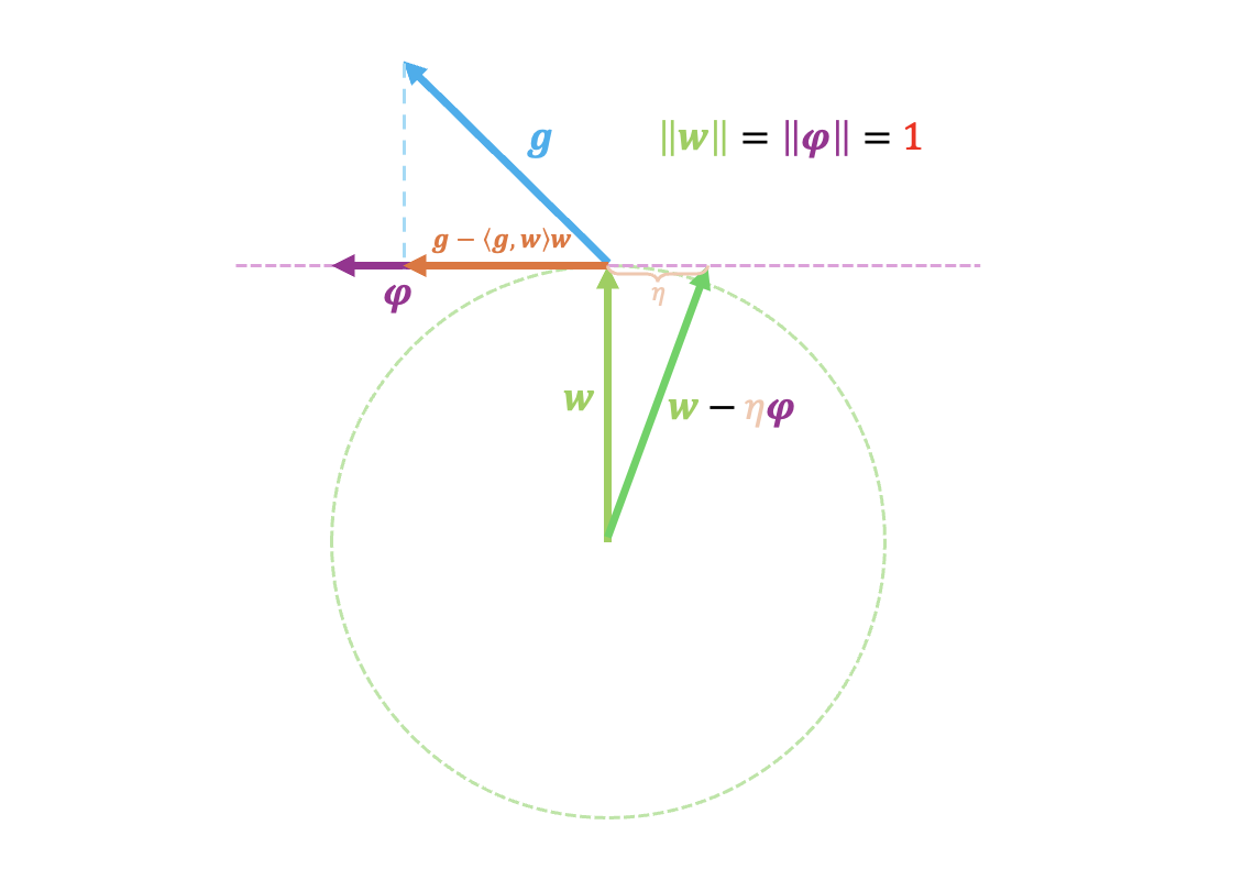Steepest descent on the sphere - geometric meaning

I believe many readers enjoy this kind of geometric perspective — it really is quite pleasing to look at. But I should remind everyone: priority should be given to carefully understanding the algebraic derivation, because a clean geometric interpretation is often more of a luxury than something you can always count on. In most cases, the complex algebra is what's actually essential.

A General Result

At this point, some readers may want to generalize this to the general $p$-norm. Let's try it together and see what difficulties arise. The problem now is:

\begin{equation}\max_{\boldsymbol{\varphi}} \langle\boldsymbol{g},\boldsymbol{\varphi}\rangle \qquad \text{s.t.}\qquad \Vert\boldsymbol{\varphi}\Vert_p = 1,\,\,\Vert\boldsymbol{w}-\eta\boldsymbol{\varphi}\Vert_p = 1,\,\,\Vert\boldsymbol{w}\Vert_p=1\end{equation}

The first-order approximation converts $\Vert\boldsymbol{w}-\eta\boldsymbol{\varphi}\Vert_p = 1$ into $\langle\boldsymbol{w}^{[p-1]},\boldsymbol{\varphi}\rangle = 0$, and then we introduce the undetermined coefficient $\lambda$:

\begin{equation}\langle\boldsymbol{g},\boldsymbol{\varphi}\rangle = \langle\boldsymbol{g},\boldsymbol{\varphi}\rangle + \lambda\langle\boldsymbol{w}^{[p-1]},\boldsymbol{\varphi}\rangle = \langle \boldsymbol{g} + \lambda\boldsymbol{w}^{[p-1]},\boldsymbol{\varphi}\rangle \leq \Vert\boldsymbol{g} + \lambda\boldsymbol{w}^{[p-1]}\Vert_q \Vert\boldsymbol{\varphi}\Vert_p = \Vert\boldsymbol{g} + \lambda\boldsymbol{w}^{[p-1]}\Vert_q \end{equation}

The condition for equality is

\begin{equation}\boldsymbol{\varphi} = \frac{(\boldsymbol{g} + \lambda\boldsymbol{w}^{[p-1]})^{[q/p]}}{\Vert(\boldsymbol{g} + \lambda\boldsymbol{w}^{[p-1]})^{[q/p]}\Vert_p}\end{equation}

Up to this point, there's been no real difficulty. However, next we need to find $\lambda$ such that $\langle\boldsymbol{w}^{[p-1]},\boldsymbol{\varphi}\rangle = 0$, and when $p \neq 2$, this is a complicated nonlinear equation with no good closed-form solution method (of course, once we do solve it, we're guaranteed to have the optimal solution, thanks to the Hölder inequality). So, for the general case of $p$, we can only stop here for now, and when we encounter concrete instances of $p\neq 2$ we'll look for numerical solution methods at that time.

That said, besides $p=2$, we can also try to solve $p\to\infty$. In this case $\boldsymbol{\varphi}=\sign(\boldsymbol{g} + \lambda\boldsymbol{w}^{[p-1]})$, and the condition $\Vert\boldsymbol{w}\Vert_p=1$ tells us the maximum value of $|w_1|,|w_2|,\cdots,|w_n|$ equals 1. If we further assume there's only a single maximum, then $\boldsymbol{w}^{[p-1]}$ is a one-hot vector, with the position of the largest absolute value being $\pm 1$ and all other entries zero. In this case we can solve for $\lambda$, and the result is that the gradient at the position of the maximum value gets clipped to zero.

Summary

This article launches a new series centered on "equality constraints" in optimization problems, attempting to find the "direction of fastest descent" for some common constraint conditions. As the first installment, this article discussed a variant of SGD under the "hypersphere" constraint.