Muon Sequel: Why Did We Choose to Try Muon?

Muon续集：为什么我们选择尝试Muon？ 苏剑林 · 2025-02-27 · Machine Learning matrix gradient optimizer spectral norm muon

This post walks through our latest technical report, Muon is Scalable for LLM Training, which shares a fairly large-scale practical run of the Muon optimizer that we previously introduced in Muon Optimizer Appreciation: A Fundamental Leap from Vectors to Matrices. We've also open-sourced the corresponding model (which we call "Moonlight," currently a 3B/16B MoE model). We arrived at a rather striking conclusion: under our experimental setup, Muon achieves nearly 2x the training efficiency of Adam.

Muon's Scaling Law and Moonlight's MMLU performance

Optimizer work is neither a huge amount nor a trivial amount, so why did we choose Muon as our new direction to explore? For an Adam optimizer whose hyperparameters are already well-tuned, how can we quickly switch over to Muon and try it out? Once we scale the model up, how does Muon's performance compare with Adam's? Below we share our thought process.

Optimization Principles

Regarding optimizers, I actually gave a brief critique before, in Muon Optimizer Appreciation: A Fundamental Leap from Vectors to Matrices: most optimizer improvements are really just small patches. That's not to say they're worthless, but ultimately they don't leave one with a sense of deep insight or excitement.

We need to start from principles that are closer to the essence of the matter, in order to think about what makes a good optimizer. Intuitively, an ideal optimizer should have two properties: stability and speed. Concretely, the update at each step of an ideal optimizer should satisfy two conditions: 1. it perturbs the model as little as possible; 2. it contributes as much as possible to reducing the loss. Put more directly: we don't want to drastically alter the model (stability), but we do want to drastically reduce the loss (speed) — a classic case of "wanting both."

How do we turn these two properties into mathematical language? Stability can be understood as a constraint on the magnitude of the update, while speed can be understood as finding the update that makes the loss function decrease the fastest. So this can be turned into a constrained optimization problem. Reusing our earlier notation, for a matrix parameter $\boldsymbol{W}\in\mathbb{R}^{n\times m}$ with gradient $\boldsymbol{G}\in\mathbb{R}^{n\times m}$, when the parameter changes from $\boldsymbol{W}$ to $\boldsymbol{W}+\Delta\boldsymbol{W}$, the change in the loss function is

\begin{equation}\text{Tr}(\boldsymbol{G}^{\top}\Delta\boldsymbol{W})\end{equation}

Then, seeking the fastest update subject to the stability constraint can be expressed as

\begin{equation}\mathop{\text{argmin}}_{\Delta\boldsymbol{W}}\text{Tr}(\boldsymbol{G}^{\top}\Delta\boldsymbol{W})\quad\text{s.t.}\quad \rho(\Delta\boldsymbol{W})\leq \eta\label{eq:least-action}\end{equation}

Here $\rho(\Delta\boldsymbol{W})\geq 0$ is some metric of stability — the smaller it is, the more stable — and $\eta$ is some constant less than 1, representing our requirement on stability; later we'll see that it is in fact the learning rate of the optimizer. If readers don't mind, borrowing a term from theoretical physics, we might call the above principle the "Least Action Principle" of optimizers.

Matrix Norms

The only thing left undetermined in equation $\eqref{eq:least-action}$ is the stability metric $\rho(\Delta\boldsymbol{W})$. Once $\rho(\Delta\boldsymbol{W})$ is chosen, $\Delta\boldsymbol{W}$ can be explicitly solved for (at least in principle). In a sense, we could say that the essential difference between different optimizers lies precisely in how they define stability.

Many readers, when first learning about SGD, have probably seen a statement like "the negative gradient direction is the direction of steepest local descent of the function value." Viewed through the framework here, this is really just choosing the stability metric to be the $F$ norm $\Vert\Delta\boldsymbol{W}\Vert_F$ of the matrix. In other words, the "direction of steepest descent" isn't fixed once and for all — it can only be pinned down after choosing a metric, and with a different norm it may no longer be the negative gradient direction.

The next natural question is: which norm most appropriately measures stability? If we impose a strong constraint, stability is assured, but the optimizer will struggle to make progress and may only converge to a suboptimal solution; conversely, if we relax the constraint, the optimizer runs wild and the training process becomes highly uncontrollable. So ideally we want to find the most precise indicator of stability. Given that neural networks are dominated by matrix multiplication, let's take $\boldsymbol{y}=\boldsymbol{x}\boldsymbol{W}$ as an example:

\begin{equation}\Vert\Delta \boldsymbol{y}\Vert = \Vert\boldsymbol{x}(\boldsymbol{W} + \Delta\boldsymbol{W}) - \boldsymbol{x}\boldsymbol{W}\Vert = \Vert\boldsymbol{x} \Delta\boldsymbol{W}\Vert\leq \rho(\Delta\boldsymbol{W}) \Vert\boldsymbol{x}\Vert\end{equation}

The above means that when the parameter changes from $\boldsymbol{W}$ to $\boldsymbol{W}+\Delta\boldsymbol{W}$, the change in the model's output is $\Delta\boldsymbol{y}$, and we hope that the magnitude of this change can be controlled by some function $\rho(\Delta\boldsymbol{W})$ related to $\Vert\boldsymbol{x}\Vert$ and $\Delta\boldsymbol{W}$; we use this function as our stability metric. From linear algebra, we know that the most precise value of $\rho(\Delta\boldsymbol{W})$ is the spectral norm $\Vert\Delta\boldsymbol{W}\Vert_2$ of $\Delta\boldsymbol{W}$. Substituting into equation $\eqref{eq:least-action}$ gives

\begin{equation}\mathop{\text{argmin}}_{\Delta\boldsymbol{W}}\text{Tr}(\boldsymbol{G}^{\top}\Delta\boldsymbol{W})\quad\text{s.t.}\quad \Vert\Delta\boldsymbol{W}\Vert_2\leq \eta\end{equation}

Solving this optimization problem yields the Muon update for $\beta=0$:

\begin{equation}\Delta\boldsymbol{W} = -\eta\, \text{msign}(\boldsymbol{G}) = -\eta\,\boldsymbol{U}_{[:,:r]}\boldsymbol{V}_{[:,:r]}^{\top}, \quad \boldsymbol{U},\boldsymbol{\Sigma},\boldsymbol{V}^{\top} = \mathop{\text{SVD}}(\boldsymbol{G})\end{equation}

When $\beta > 0$, $\boldsymbol{G}$ is replaced with the momentum $\boldsymbol{M}$, and $\boldsymbol{M}$ can be viewed as a smoother estimate of the gradient, so it can still be understood as following from the equation above. Hence we can state that "Muon is precisely steepest descent under the spectral norm," while things like the Newton–Schulz iteration are simply computational approximations to it — we won't go into detail here. We already gave the detailed derivation in Muon Optimizer Appreciation: A Fundamental Leap from Vectors to Matrices, so we won't repeat it.

Weight Decay

At this point we can answer the first question: why did we choose to try Muon? Because, like SGD, Muon gives the direction of steepest descent, but its spectral-norm constraint is more precise than SGD's $F$-norm constraint, giving it greater potential. From another angle, improving optimizers by "choosing the most suitable constraint for different parameters" also seems more fundamental than the usual patchwork of ad hoc modifications.

Of course, potential doesn't guarantee actual performance, and there are some "traps" involved in verifying Muon on larger-scale models. The first issue we ran into was weight decay. Although we included weight decay when introducing Muon in Muon Optimizer Appreciation: A Fundamental Leap from Vectors to Matrices, the original authors' version of Muon actually did not have it, and we initially followed the official version too. The result was that Muon converged quickly at first, but Adam soon caught up, and various "internal signs" even showed hints of collapse.

We quickly realized this was likely a weight decay issue, so we added it back:

\begin{equation}\Delta\boldsymbol{W} = -\eta\, [\text{msign}(\boldsymbol{M})+ \lambda \boldsymbol{W}]\end{equation}

Running the experiment again, sure enough, this time Muon stayed ahead of Adam throughout, as shown in Figure 2 of the paper:

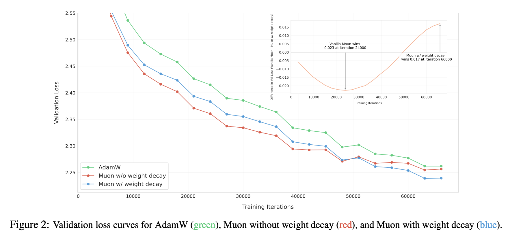Comparison of results with and without weight decay

What role does weight decay play? Looking back at it, the key point is likely that it keeps the parameter norm bounded:

\begin{equation}\begin{aligned} \Vert\boldsymbol{W}_t\Vert =&\, \Vert\boldsymbol{W}_{t-1} - \eta_t (\boldsymbol{\Phi}_t + \lambda \boldsymbol{W}_{t-1})\Vert \\[5pt] =&\, \Vert(1 - \eta_t \lambda)\boldsymbol{W}_{t-1} - \eta_t \lambda (\boldsymbol{\Phi}_t/\lambda)\Vert \\[5pt] \leq &\,(1 - \eta_t \lambda)\Vert\boldsymbol{W}_{t-1}\Vert + \eta_t \lambda \Vert\boldsymbol{\Phi}_t/\lambda\Vert \\[5pt] \leq &\,\max(\Vert\boldsymbol{W}_{t-1}\Vert,\Vert\boldsymbol{\Phi}_t/\lambda\Vert) \\[5pt] \end{aligned}\end{equation}

Here $\Vert\cdot\Vert$ is any matrix norm, i.e., the inequality above holds for any matrix norm, and $\boldsymbol{\Phi}_t$ is the update vector given by the optimizer — for Muon this is $\text{msign}(\boldsymbol{M})$. When we take the spectral norm, we have $\Vert\text{msign}(\boldsymbol{M})\Vert_2 = 1$, so for Muon we get

\begin{equation} \Vert\boldsymbol{W}_t\Vert_2 \leq \max(\Vert\boldsymbol{W}_{t-1}\Vert_2,1/\lambda)\leq\cdots \leq \max(\Vert\boldsymbol{W}_0\Vert_2,1/\lambda)\end{equation}

This ensures the model's "internal health," because $\Vert\boldsymbol{x}\boldsymbol{W}\Vert\leq \Vert\boldsymbol{x}\Vert\Vert\boldsymbol{W}\Vert_2$ is controlled, so $\Vert\boldsymbol{W}\Vert_2$ is also controlled, which in turn means $\Vert\boldsymbol{x}\boldsymbol{W}\Vert$ is controlled, avoiding the risk of blow-up — this is especially important for issues such as exploding attention logits. Of course, in most cases this bound is quite loose in practice; the actual spectral norm of the parameters is typically far below this bound. This inequality is only meant to illustrate that weight decay has the property of controlling the norm.

RMS Alignment

When we decide to try a new optimizer, one thorny issue is how to quickly find near-optimal hyperparameters. Muon, for instance, has at least two hyperparameters: the learning rate $\eta_t$ and the decay rate $\lambda$. Grid search is of course an option, but it's time-consuming and laborious. Here we propose an Update RMS Alignment approach for hyperparameter transfer, which lets us carry over hyperparameters already tuned for Adam to other optimizers.

First, for a matrix $\boldsymbol{W}\in\mathbb{R}^{n\times m}$, its RMS (Root Mean Square) is defined as

\begin{equation}\text{RMS}(\boldsymbol{W}) = \frac{\Vert \boldsymbol{W}\Vert_F}{\sqrt{nm}} = \sqrt{\frac{1}{nm}\sum_{i=1}^n\sum_{j=1}^m W_{i,j}^2}\end{equation}

In short, RMS measures the average magnitude of the elements of a matrix. We observed that the RMS of Adam's updates is quite stable, typically between 0.2 and 0.4, which is also why theoretical analyses often use SignSGD as an approximation to Adam. Based on this, we propose aligning the update RMS of the new optimizer to 0.2 via RMS normalization:

\begin{gather} \boldsymbol{W}_t =\boldsymbol{W}_{t-1} - \eta_t (\boldsymbol{\Phi}_t + \lambda \boldsymbol{W}_{t-1}) \\[6pt] \downarrow \notag\\[6pt] \boldsymbol{W}_t = \boldsymbol{W}_{t-1} - \eta_t (0.2\, \boldsymbol{\Phi}_t/\text{RMS}(\boldsymbol{\Phi}_t) + \lambda \boldsymbol{W}_{t-1}) \end{gather}

This way we can reuse Adam's $\eta_t$ and $\lambda$, achieving roughly the same per-step update magnitude for the parameters. In practice, this simple strategy for migrating from Adam to Muon already yields results clearly better than Adam, close to what you'd get from a further fine-grained hyperparameter search for Muon. In particular, Muon's $\text{RMS}(\boldsymbol{\Phi}_t)=\text{RMS}(\boldsymbol{U}_{[:,:r]}\boldsymbol{V}_{[:,:r]}^{\top})$ can even be computed analytically:

\begin{equation}nm\,\text{RMS}(\boldsymbol{\Phi}_t)^2 = \sum_{i=1}^n\sum_{j=1}^m \sum_{k=1}^r U_{i,k}^2V_{k,j}^2 = \sum_{k=1}^r\left(\sum_{i=1}^n U_{i,k}^2\right)\left(\sum_{j=1}^m V_{k,j}^2\right) = \sum_{k=1}^r 1 = r\end{equation}

That is, $\text{RMS}(\boldsymbol{\Phi}_t) = \sqrt{r/nm}$. In practice, the probability that a matrix is strictly low-rank is small, so we can take $r = \min(n,m)$, and hence $\text{RMS}(\boldsymbol{\Phi}_t) = \sqrt{1/\max(n,m)}$. So in the end we didn't use RMS normalization directly, but instead used this equivalent analytic form:

\begin{equation}\boldsymbol{W}_t = \boldsymbol{W}_{t-1} - \eta_t (0.2\, \boldsymbol{\Phi}_t\,\sqrt{\max(n,m)} + \lambda \boldsymbol{W}_{t-1})\end{equation}

This final formula shows that it is not appropriate to use a single shared learning rate for all parameters in Muon. For instance, Moonlight is an MoE model with many matrix parameters that deviate considerably from being square, so $\max(n,m)$ varies substantially. Using a single learning rate would inevitably cause some parameters to update too fast or too slow relative to others, hurting the final performance.

Experimental Analysis

On this 2.4B/16B-scale MoE model, we conducted a fairly thorough comparison between Adam and Muon, and found that Muon has a clear advantage both in convergence speed and final performance. For detailed comparisons, please refer to the original paper — here we only share a selection.

GitHub: https://github.com/MoonshotAI/Moonlight

First, here's a relatively objective comparison table, including our own controlled comparison between Muon and Adam, as well as a comparison against an externally trained model (DeepSeek) with the same architecture trained using Adam (to facilitate comparison, Moonlight's architecture is identical to DSV3-Small), showing Muon's distinct advantage:

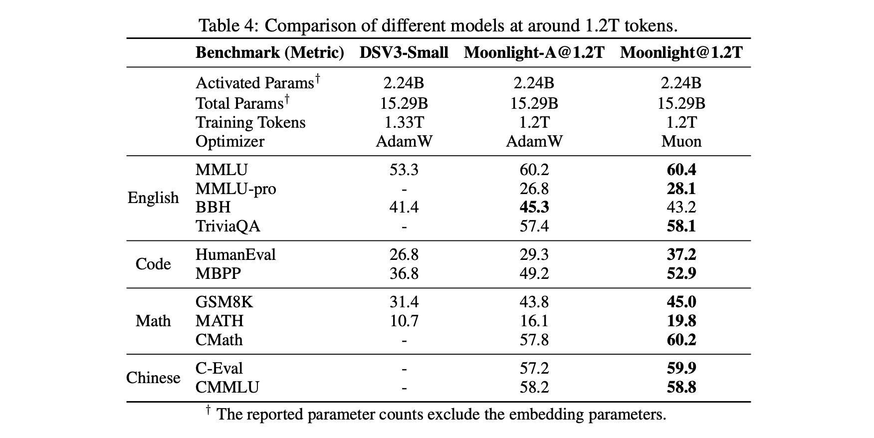Comparison of Muon (Moonlight) vs. Adam (Moonlight-A and DSV3-small)

What's different about models trained with Muon? Since we said earlier that Muon performs steepest descent under the spectral norm — and the spectral norm is the largest singular value — this led us to monitor and analyze the singular values. Sure enough, we found some interesting signals: parameters trained with Muon have a more uniform singular value distribution. We use singular value entropy to quantify this phenomenon:

\begin{equation}H(\boldsymbol{\sigma}) = -\frac{1}{\log n}\sum_{i=1}^n \frac{\sigma_i^2}{\sum_{j=1}^n\sigma_j^2}\log \frac{\sigma_i^2}{\sum_{j=1}^n\sigma_j^2}\end{equation}

Here $\boldsymbol{\sigma}=(\sigma_1,\sigma_2,\cdots,\sigma_n)$ denotes the full set of singular values of a given parameter. Parameters trained with Muon have higher entropy, i.e., a more uniform singular value distribution, meaning this parameter is harder to compress — indicating that Muon makes fuller use of the parameter's potential:

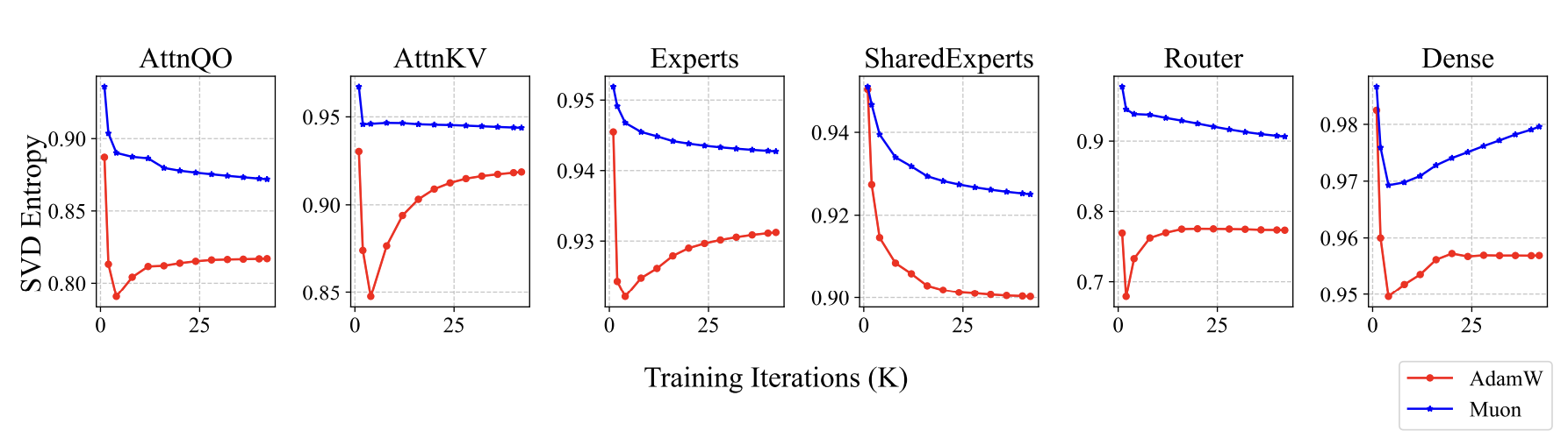Weights trained with Muon have higher singular-value entropy

Another interesting finding is that when we apply Muon to fine-tuning (SFT), we may end up in a suboptimal solution if pretraining did not use Muon. Specifically, if both pretraining and fine-tuning use Muon, performance is best; but among the other three combinations (Adam+Muon, Muon+Adam, Adam+Adam), no clear pattern emerges regarding which is better or worse.

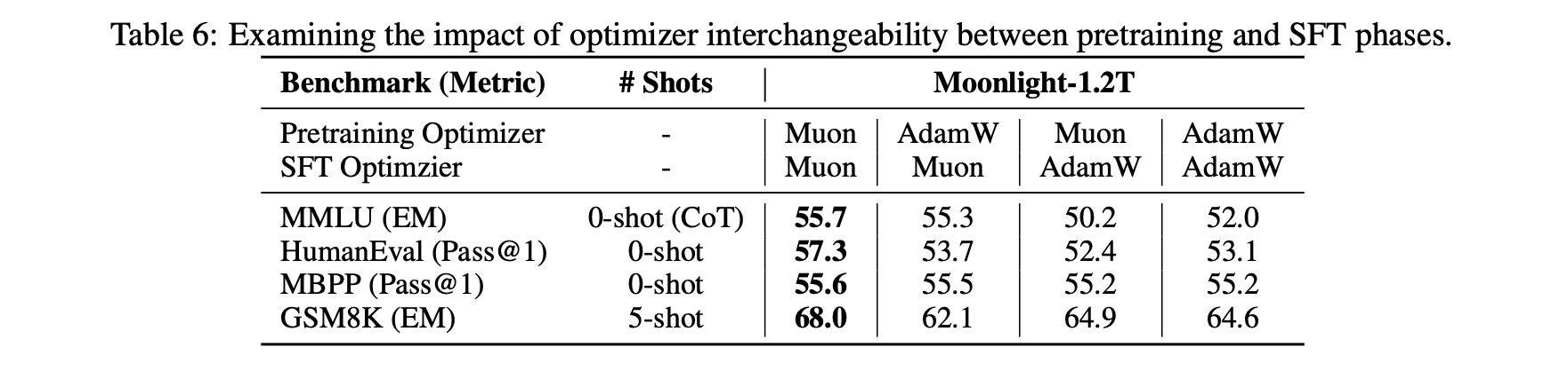Testing combinations of Muon/Adam for pretraining/fine-tuning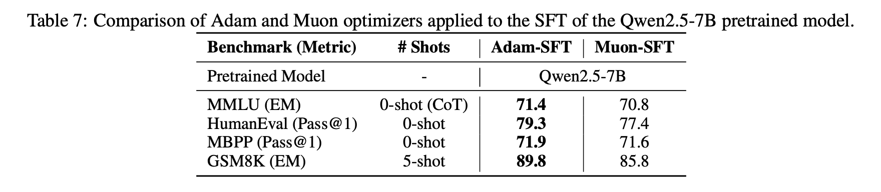Attempts at fine-tuning open-source models with Muon/Adam

This phenomenon suggests that certain special initializations are unfavorable to Muon; conversely, there might also exist initializations that are especially favorable to Muon. We're still exploring the deeper underlying principles.

Further Thoughts

Overall, in our experiments, Muon's performance compares very favorably with Adam's. As a new optimizer whose form differs substantially from Adam's, this performance is not merely "commendable" — it also suggests that Muon may be capturing something essential.

There's a view that has circulated in the community: Adam performs well partly because mainstream model architecture improvements have been "overfitting" to Adam. This view seems to originate from Neural Networks (Maybe) Evolved to Make Adam The Best Optimizer. It might sound a bit absurd at first, but there's real substance to it. Think about it: whenever we try to improve a model, we train it with Adam to see how it performs — if it performs well, we keep the change; if not, we discard it. But is that good performance really because the change is inherently better, or because it happens to be a better match for Adam?

This is worth pondering. Not to say it applies to everything, but at least some fraction of such work surely owes its apparent improvement to being a better fit for Adam, and over time, model architectures gradually evolve in directions favorable to Adam. Against this backdrop, the fact that an optimizer so different from Adam can still "break out" is especially noteworthy. Note that neither I nor my company are affiliated with the people who proposed Muon, so these remarks are purely "heartfelt opinions" and not self-promotion.

What further work remains to be done on Muon? Probably quite a lot. For instance, the issue mentioned above — poor results from "Adam pretraining + Muon fine-tuning" — deserves further analysis, since practically all publicly released model weights today are trained with Adam; if Muon fine-tuning doesn't work well on them, that will inevitably hinder its adoption. Of course, this also gives us an opportunity to deepen our understanding of Muon (learning by debugging).

There's also a broader line of thought: Muon is based on the spectral norm, which is the largest singular value, but in fact we can construct a whole family of norms based on singular values, such as the Schatten norms. Generalizing Muon to this broader class of norms and then tuning accordingly could, in principle, yield even better results. In addition, after Moonlight's release, some readers asked how µP (maximal update parametrization) should be designed under Muon — this is also a pressing open question.

Summary

This post introduced our fairly large-scale practical exploration of the Muon optimizer (Moonlight), and shared our latest thoughts on the Muon optimizer.