Diffusion Models Chat (27): Using Step Size as a Conditioning Input

生成扩散模型漫谈（二十七）：将步长作为条件输入 苏剑林 · 2024-12-15 · Machine Learning differential equation generative model sampling diffusion

This article once again focuses on accelerating sampling for diffusion models. As is well known, there are two main approaches to accelerating diffusion model sampling: developing more efficient solvers, or post-hoc distillation. However, as far as the author can tell, apart from SiD introduced in the previous two posts, neither approach has often managed to reduce the number of generation steps down to one. While SiD does achieve single-step generation, it requires additional distillation costs, and the distillation process involves a GAN-like alternating training procedure, which always feels somewhat unsatisfying.

This article introduces One Step Diffusion via Shortcut Models, whose breakthrough idea is to also feed the generation step size into the diffusion model as a conditioning input, and then add an intuitive regularization term to the training objective. This makes it possible to directly and stably train a model capable of single-step generation—a simple yet effective classic piece of work.

ODE-Based Diffusion

The conclusions in the original paper are based on ODE-style diffusion models. We've introduced the theoretical foundations of ODE-style diffusion many times in this series, in posts (6), (12), (14), (15), and (17). Perhaps the simplest way to understand it is the ReFlow perspective from (17), which we briefly recap below. more

Suppose $\boldsymbol{x}_0\sim p_0(\boldsymbol{x}_0)$ is random noise sampled from the prior distribution, and $\boldsymbol{x}_1\sim p_1(\boldsymbol{x}_1)$ is a real sample drawn from the target distribution (note: in earlier posts, the usual convention was that $\boldsymbol{x}_T$ denotes noise and $\boldsymbol{x}_0$ denotes the target sample; here, for convenience, we've swapped them). ReFlow allows us to specify an arbitrary trajectory of motion from $\boldsymbol{x}_0$ to $\boldsymbol{x}_1$, the simplest of which is naturally a straight line:

\begin{equation}\boldsymbol{x}_t = (1-t)\boldsymbol{x}_0 + t \boldsymbol{x}_1\label{eq:line}\end{equation}

Differentiating both sides gives us the ODE it satisfies:

\begin{equation}\frac{d\boldsymbol{x}_t}{dt} = \boldsymbol{x}_1 - \boldsymbol{x}_0\end{equation}

This ODE is simple, but not actually useful in practice, because what we want is to generate $\boldsymbol{x}_1$ from $\boldsymbol{x}_0$ via the ODE, whereas the above ODE explicitly depends on $\boldsymbol{x}_1$. To resolve this, a straightforward idea is to "learn a function of $\boldsymbol{x}_t$ that approximates $\boldsymbol{x}_1 - \boldsymbol{x}_0$," and then, once learned, use it in place of $\boldsymbol{x}_1 - \boldsymbol{x}_0$, i.e.,

\begin{equation}\boldsymbol{\theta}^* = \mathop{\text{argmin}}_{\boldsymbol{\theta}} \mathbb{E}_{\boldsymbol{x}_0\sim p_0(\boldsymbol{x}_0),\boldsymbol{x}_1\sim p_1(\boldsymbol{x}_1)}\left[\Vert\boldsymbol{v}_{\boldsymbol{\theta}}(\boldsymbol{x}_t, t) - (\boldsymbol{x}_1 - \boldsymbol{x}_0)\Vert^2\right]\label{eq:loss}\end{equation}

and

\begin{equation}\frac{d\boldsymbol{x}_t}{dt} = \boldsymbol{x}_1 - \boldsymbol{x}_0\quad\Rightarrow\quad\frac{d\boldsymbol{x}_t}{dt} = \boldsymbol{v}_{\boldsymbol{\theta}^*}(\boldsymbol{x}_t, t)\label{eq:ode-core}\end{equation}

This is ReFlow. Of course, there's a theoretical gap left here—namely, whether the ODE obtained by fitting $\boldsymbol{v}_{\boldsymbol{\theta}}(\boldsymbol{x}_t, t)$ via squared error indeed generates the distribution we expect. Readers can consult Diffusion Models Chat (17): General Steps for Constructing ODEs (Part 2) for that part.

Step-Size Self-Consistency

Suppose we already have $\boldsymbol{v}_{\boldsymbol{\theta}}(\boldsymbol{x}_t, t)$; then solving the differential equation $\frac{d\boldsymbol{x}_t}{dt} = \boldsymbol{v}_{\boldsymbol{\theta}}(\boldsymbol{x}_t, t)$ lets us transform from $\boldsymbol{x}_0$ to $\boldsymbol{x}_1$. The key word here is "differential equation"—but in practice we can't actually numerically compute a differential equation, only a "difference equation":

\begin{equation}\boldsymbol{x}_{t + \epsilon} - \boldsymbol{x}_t = \boldsymbol{v}_{\boldsymbol{\theta}}(\boldsymbol{x}_t, t) \epsilon\label{eq:de}\end{equation}

This difference equation is the "Euler approximation" of the original ODE, and its accuracy depends on the size of the step $\epsilon$; when $\epsilon\to 0$, it becomes exactly equal to the original ODE—in other words, the smaller the step, the more accurate it is. However, the number of generation steps equals $1/\epsilon$, and we want as few generation steps as possible, which means we can't use too small a step—ideally $\epsilon$ could equal 1, so that $\boldsymbol{x}_1 = \boldsymbol{x}_0 + \boldsymbol{v}_{\boldsymbol{\theta}}(\boldsymbol{x}_0, 0)$ and generation could be completed in a single step.

The problem is that if we plug a large step size directly into the above formula, the resulting $\boldsymbol{x}_1$ will inevitably deviate severely from the exact solution. This is where the clever design of the original paper (hereafter called the "Shortcut model") comes into play: it argues that the model $\boldsymbol{v}_{\boldsymbol{\theta}}(\boldsymbol{x}_t, t)$ shouldn't just be a function of $\boldsymbol{x}_t$ and $t$, but should also be a function of the step size $\epsilon$, so that the difference equation $\eqref{eq:de}$ can adapt itself to the step size:

\begin{equation}\boldsymbol{x}_{t + \epsilon} - \boldsymbol{x}_t = \boldsymbol{v}_{\boldsymbol{\theta}}(\boldsymbol{x}_t, t, \epsilon) \epsilon\end{equation}

The objective $\eqref{eq:loss}$ trains an exact ODE model, so it trains the model for $\epsilon=0$:

\begin{equation}\mathcal{L}_1 = \mathbb{E}_{\boldsymbol{x}_0\sim p_0(\boldsymbol{x}_0),\boldsymbol{x}_1\sim p_1(\boldsymbol{x}_1)}\left[\frac{1}{2}\Vert\boldsymbol{v}_{\boldsymbol{\theta}}(\boldsymbol{x}_t, t, 0) - (\boldsymbol{x}_1 - \boldsymbol{x}_0)\Vert^2\right]\end{equation}

So how is the $\epsilon > 0$ part trained? Our goal is to make the number of generation steps as small as possible, which is equivalent to requiring that "taking one step of twice the step size equals taking two steps of the original step size":

\begin{equation}\boldsymbol{x}_t + \boldsymbol{v}_{\boldsymbol{\theta}}(\boldsymbol{x}_t, t, 2\epsilon) 2\epsilon = \color{green}{\underbrace{\boldsymbol{x}_t + \boldsymbol{v}_{\boldsymbol{\theta}}(\boldsymbol{x}_t, t, \epsilon) \epsilon}_{\tilde{\boldsymbol{x}}_{t+\epsilon}}} + \boldsymbol{v}_{\boldsymbol{\theta}}\big(\color{green}{\underbrace{\boldsymbol{x}_t + \boldsymbol{v}_{\boldsymbol{\theta}}(\boldsymbol{x}_t, t, \epsilon) \epsilon}_{\tilde{\boldsymbol{x}}_{t+\epsilon}}}, t+\epsilon, \epsilon\big) \epsilon\label{eq:cond}\end{equation}

That is, $\boldsymbol{v}_{\boldsymbol{\theta}}(\boldsymbol{x}_t, t, 2\epsilon) = [\boldsymbol{v}_{\boldsymbol{\theta}}(\boldsymbol{x}_t, t, \epsilon) + \boldsymbol{v}_{\boldsymbol{\theta}}(\color{green}{\tilde{\boldsymbol{x}}_{t+\epsilon}}, t+\epsilon, \epsilon)] /2$. To achieve this goal, we add a self-consistency loss function:

\begin{equation}\mathcal{L}_2 = \mathbb{E}_{\boldsymbol{x}_0\sim p_0(\boldsymbol{x}_0),\boldsymbol{x}_1\sim p_1(\boldsymbol{x}_1)}\left[\Vert\boldsymbol{v}_{\boldsymbol{\theta}}(\boldsymbol{x}_t, t, 2\epsilon) - [\boldsymbol{v}_{\boldsymbol{\theta}}(\boldsymbol{x}_t, t, \epsilon)+ \boldsymbol{v}_{\boldsymbol{\theta}}(\color{green}{\tilde{\boldsymbol{x}}_{t+\epsilon}}, t+\epsilon, \epsilon) ]/2\Vert^2\right]\end{equation}

Adding $\mathcal{L}_1$ and $\mathcal{L}_2$ together gives us the loss function of the Shortcut model.

(Note: as one reader pointed out, the earlier work Consistency Trajectory Models: Learning Probability Flow ODE Trajectory of Diffusion had already proposed conditioning on the discretized start and end times; once the start and end are specified, the step size is effectively determined too. So the Shortcut model's approach of conditioning on step size isn't entirely novel.)

Model Details

The above is essentially the entire theoretical content of the Shortcut model—very elegant and concise. But going from theory to experiment still requires some details, such as how the step size $\epsilon$ is incorporated into the model.

First, when training $\mathcal{L}_2$, Shortcut doesn't sample $\epsilon$ uniformly from $[0,1]$. Instead, it sets a minimum step size $2^{-7}$, and then doubles it repeatedly up to 1, so that all nonzero step sizes take only these 8 values: $\{2^{-7},2^{-6},2^{-5},2^{-4},2^{-3},2^{-2},2^{-1},1\}$. It uniformly samples from the first 7 to train $\mathcal{L}_2$. This means the possible values of $\epsilon$ are finite—counting $0$, there are only 9 in total—so the Shortcut model feeds in $\epsilon$ directly as an embedding, adding it to the embedding of $t$.

Second, note that computing $\mathcal{L}_2$ is more expensive than computing $\mathcal{L}_1$, since the term $\boldsymbol{v}_{\boldsymbol{\theta}}(\tilde{\boldsymbol{x}}_{t+\epsilon}, t, \epsilon)$ requires two forward passes. So the paper's approach is to use, within each batch, $3/4$ of the samples to compute $\mathcal{L}_1$, and the remaining $1/4$ samples to compute $\mathcal{L}_2$. This not only saves computation but also effectively adjusts the weighting of $\mathcal{L}_1,\mathcal{L}_2$, since $\mathcal{L}_2$ is easier to train than $\mathcal{L}_1$ and so can be given proportionally fewer training samples.

Additionally, in practice the paper also makes a small tweak to $\mathcal{L}_2$, adding a stop-gradient operator:

\begin{equation}\mathcal{L}_2 = \mathbb{E}_{\boldsymbol{x}_0\sim p_0(\boldsymbol{x}_0),\boldsymbol{x}_1\sim p_1(\boldsymbol{x}_1)}\left[\Vert\boldsymbol{v}_{\boldsymbol{\theta}}(\boldsymbol{x}_t, t, 2\epsilon) - \color{skyblue}{\text{sg}[}\boldsymbol{v}_{\boldsymbol{\theta}}(\boldsymbol{x}_t, t, \epsilon)+ \boldsymbol{v}_{\boldsymbol{\theta}}(\color{green}{\tilde{\boldsymbol{x}}_{t+\epsilon}}, t+\epsilon, \epsilon) \color{skyblue}{]}/2\Vert^2\right]\end{equation}

Why do this? According to the author's reply, this is a common practice in self-bootstrapped learning: the part under stop-gradient serves as a target and shouldn't receive gradients, similar to unsupervised learning schemes like BYOL and SimSiam. However, in the author's opinion, the biggest value of this operation is really saving on training cost, since the term $\boldsymbol{v}_{\boldsymbol{\theta}}(\tilde{\boldsymbol{x}}_{t+\epsilon}, t, \epsilon)$ already requires two forward passes—backpropagating through it as well would double the computation again.

Experimental Results

Now let's look at the experimental results of the Shortcut model. It appears to currently be the best single-stage-trained diffusion model for single-step generation:

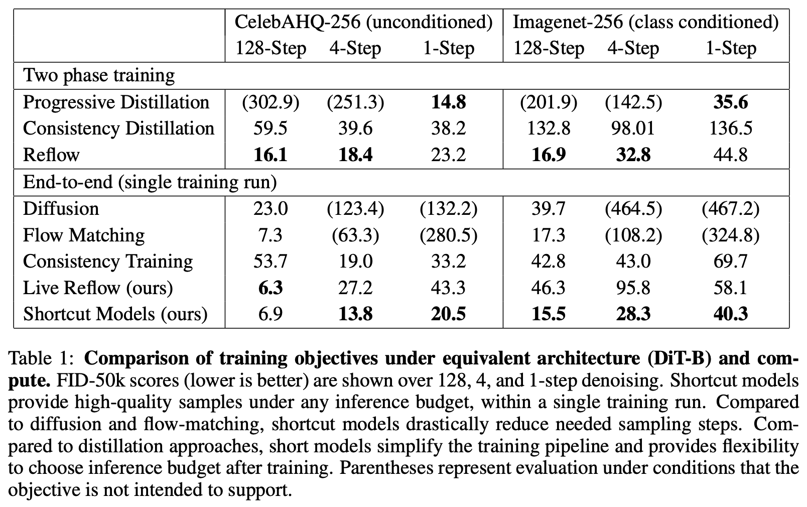Generation quality evaluation of various diffusion models

Here's a comparison of its actual sampling results:

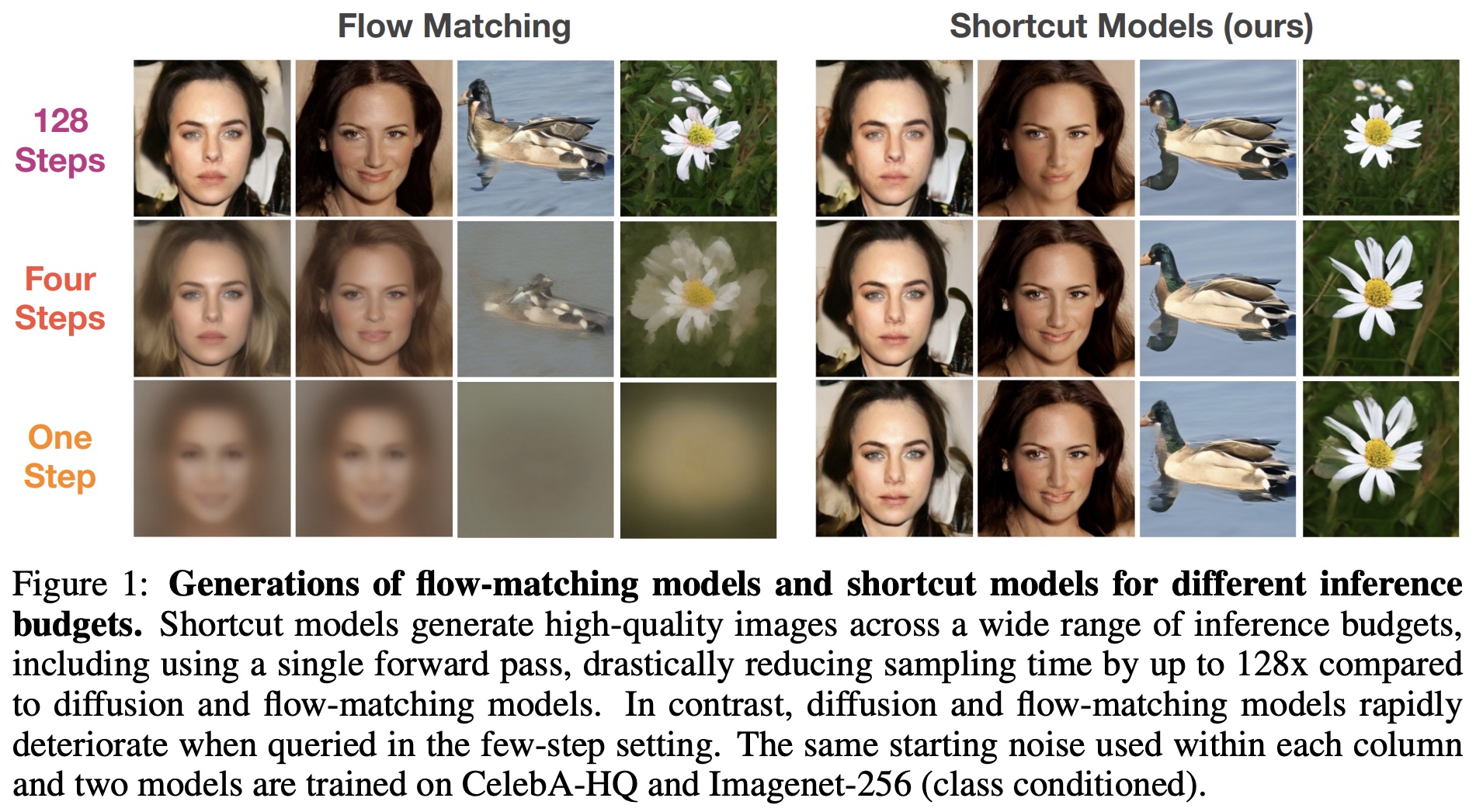Comparison of actual sampling results between Flow Matching and the Shortcut Model

However, on closer inspection of the single-step generated samples, one can still see obvious flaws. So while the Shortcut model represents significant progress over previous single-stage training schemes, there is still clear room for improvement.

The author has open-sourced the Shortcut model's code, available on GitHub at:

https://github.com/kvfrans/shortcut-models

Incidentally, the Shortcut model was submitted to ICLR 2025 and received unanimously positive reviews (a perfect score of 8 across the board).

Further Reflections

Reading about the Shortcut model, one wonders what related work comes to mind for readers. The author was reminded of something perhaps unexpected: AMED, which we introduced in Diffusion Models Chat (21): Accelerating ODE Sampling via the Mean Value Theorem.

The Shortcut model and AMED share the same underlying idea: both have discovered that simply studying complex higher-order solvers can already easily reduce the generation NFE (number of function evaluations, i.e., model runs) down to single digits—let alone achieving single-step generation. So both agree that what really needs to change isn't the solver, but the model itself. How should it change? AMED's answer is the "mean value theorem": integrating both sides of the ODE, we have the exact expression

\begin{equation}\boldsymbol{x}_{t + \epsilon} - \boldsymbol{x}_t = \int_t^{t + \epsilon}\boldsymbol{v}_{\boldsymbol{\theta}}(\boldsymbol{x}_{\tau}, \tau) d\tau\end{equation}

By analogy with the "mean value theorem for integrals," we can find some $s\in[t, t + \epsilon]$ such that

\begin{equation}\frac{1}{\epsilon}\int_t^{t + \epsilon}\boldsymbol{v}_{\boldsymbol{\theta}}(\boldsymbol{x}_{\tau}, \tau) d\tau = \boldsymbol{v}_{\boldsymbol{\theta}}(\boldsymbol{x}_s, s)\end{equation}

holds, giving us

\begin{equation}\boldsymbol{x}_{t + \epsilon} - \boldsymbol{x}_t = \boldsymbol{v}_{\boldsymbol{\theta}}(\boldsymbol{x}_s, s) \epsilon\end{equation}

Of course, the mean value theorem for integrals technically only holds for scalar functions, and is not guaranteed to hold for vector-valued functions—hence the qualifier "by analogy." The problem now is that we don't know the value of $s$, so AMED's subsequent approach is to use a very small model (with almost negligible compute cost) to predict $s$.

AMED is a post-hoc correction method applied to an existing diffusion model, so its effectiveness depends on how well the mean value theorem holds for the $\boldsymbol{v}_{\boldsymbol{\theta}}(\boldsymbol{x}_t, t)$ model—which involves something of a "luck factor." Moreover, AMED needs to first estimate $\boldsymbol{x}_s$ using the Euler scheme, so its minimum NFE is 2; it can't achieve single-step generation. By comparison, the Shortcut model is more "aggressive": it directly feeds the step size in as a conditioning input, and turns the condition for accelerated generation, $\eqref{eq:cond}$, into a loss function. This not only sidesteps the discussion of whether the "mean value theorem" approximation is feasible, but also allows the minimum NFE to drop to 1.

More cleverly, on closer reflection we find that the two approaches actually share some commonality. As mentioned earlier, Shortcut directly converts $\epsilon$ into an embedding and adds it to the embedding of $t$—isn't this effectively the same as AMED's modification of $t$! It's just that AMED directly modifies the numerical value of $t$, while Shortcut modifies the embedding of $t$.

Summary

This article introduced a new diffusion model that achieves single-step generation with only single-stage training. Its breakthrough idea is to feed the step size into the diffusion model as a conditioning input as well, paired with an intuitive regularization term, so that single-stage training alone suffices to obtain a diffusion model capable of single-step generation.