Transformer Upgrade Path: 18. The Choice Principle for RoPE's Base

Transformer升级之路：18、RoPE的底数选择原则 苏剑林 · 2024-05-29 · Machine Learning inequality attention positional encoding RoPE

As we know, in RoPE, the frequency computation formula is $\theta_i = b^{-2i/d}$, and the base $b$ has a default value of 10000. Currently, one of the mainstream approaches for Long Context is: first pretrain on short texts with $b=10000$, then increase $b$ and fine-tune on long texts. The rationale for this comes from the NTK-RoPE introduced in Transformer Upgrade Path: 10. RoPE as a β-ary Encoding, which itself has good length-generalization properties — switching to a larger $b$ before fine-tuning gives a lower starting loss and faster convergence compared to fine-tuning without any modification. This process gives the impression that increasing $b$ is entirely a consequence of the "short-then-long" training strategy — as if, if we trained on long texts from the start, there would be no need to increase $b$ at all?

A paper from last week, Base of RoPE Bounds Context Length, attempts to answer this question. Based on a desired property, it studies the lower bound of $b$ and points out that a larger training length should itself call for a larger base, independent of the training strategy. The overall line of analysis is quite illuminating, so let's take a look together. more

The Desired Property

We won't go into full detail on RoPE here; in essence, it's a block-diagonal matrix

\begin{equation}\boldsymbol{\mathcal{R}}_n = \scriptsize{\left(\begin{array}{cc:cc:cc:cc} \cos n\theta_0 & -\sin n\theta_0 & 0 & 0 & \cdots & \cdots & 0 & 0 \\ \sin n\theta_0 & \cos n\theta_0 & 0 & 0 & \cdots & \cdots & 0 & 0 \\ \hdashline 0 & 0 & \cos n\theta_1 & -\sin n\theta_1 & \cdots & \cdots & 0 & 0 \\ 0 & 0 & \sin n\theta_1 & \cos n\theta_1 & \cdots & \cdots & 0 & 0 \\ \hdashline \vdots & \vdots & \vdots & \vdots & \ddots & \ddots & \vdots & \vdots \\ \vdots & \vdots & \vdots & \vdots & \ddots & \ddots & \vdots & \vdots \\ \hdashline 0 & 0 & 0 & 0 & \cdots & \cdots & \cos n\theta_{d/2-1} & -\sin n\theta_{d/2-1} \\ 0 & 0 & 0 & 0 & \cdots & \cdots & \sin n\theta_{d/2-1} & \cos n\theta_{d/2-1} \\ \end{array}\right)}\end{equation}

which, using the identity

\begin{equation}(\boldsymbol{\mathcal{R}}_m \boldsymbol{q})^{\top}(\boldsymbol{\mathcal{R}}_n \boldsymbol{k}) = \boldsymbol{q}^{\top} \boldsymbol{\mathcal{R}}_m^{\top}\boldsymbol{\mathcal{R}}_n \boldsymbol{k} = \boldsymbol{q}^{\top} \boldsymbol{\mathcal{R}}_{n-m} \boldsymbol{k}\end{equation}

injects absolute position information into $\boldsymbol{q},\boldsymbol{k}$ while automatically achieving relative position effects. Here $\theta_i = b^{-2i/d}$, and the choice of value for $b$ is exactly the question this article investigates.

Besides injecting positional information into the model, we hope RoPE has two ideal properties for better performance: 1. Long-range decay, i.e., tokens that are closer together should on average receive more attention; 2. Semantic aggregation, i.e., tokens that are semantically similar should on average receive more attention. We already discussed the first point back in Transformer Upgrade Path: 2. Rotary Position Embedding, Drawing on Various Strengths, where we showed that RoPE does indeed have a certain long-range decay property.

So let's move on to analyzing the second point.

An Inequality Relation

By "semantic aggregation," we mean that when $\boldsymbol{k}$ and $\boldsymbol{q}$ are close to each other, regardless of how large their relative distance $n-m$ is, the attention $\boldsymbol{q}^{\top} \boldsymbol{\mathcal{R}}_{n-m} \boldsymbol{k}$ between them should on average be larger (at least larger than that between two random tokens). To reach a quantitative conclusion, we further simplify the problem by assuming that each component of $\boldsymbol{q}$ is i.i.d., with mean $\mu$ and variance $\sigma^2$ per component.

Now consider two different cases for $\boldsymbol{k}$: one where, starting from $\boldsymbol{q}$, we add a zero-mean perturbation $\boldsymbol{\varepsilon}$, which we denote $\tilde{\boldsymbol{k}} = \boldsymbol{q} + \boldsymbol{\varepsilon}$, representing a token semantically close to $\boldsymbol{q}$; the other where we assume $\boldsymbol{k}$ is i.i.d. with $\boldsymbol{q}$, representing two random tokens. According to the second ideal property, we would like to have

\begin{equation}\mathbb{E}_{\boldsymbol{q},\boldsymbol{k},\boldsymbol{\varepsilon}}\big[\boldsymbol{q}^{\top} \boldsymbol{\mathcal{R}}_{n-m} \tilde{\boldsymbol{k}} - \boldsymbol{q}^{\top} \boldsymbol{\mathcal{R}}_{n-m} \boldsymbol{k}\big] \geq 0\end{equation}

Note that we've repeatedly emphasized "on average," meaning we only expect this trend to hold on average, not strictly at every single point — which is why we take the expectation $\mathbb{E}_{\boldsymbol{q},\boldsymbol{k},\boldsymbol{\varepsilon}}$ on both sides above. Now, based on our assumptions and the definition of RoPE, we can work this out explicitly:

\begin{equation}\begin{aligned} &\,\mathbb{E}_{\boldsymbol{q},\boldsymbol{k},\boldsymbol{\varepsilon}}\big[\boldsymbol{q}^{\top} \boldsymbol{\mathcal{R}}_{n-m} (\boldsymbol{q} + \boldsymbol{\varepsilon}) - \boldsymbol{q}^{\top} \boldsymbol{\mathcal{R}}_{n-m} \boldsymbol{k}\big] \\[5pt] =&\, \mathbb{E}_{\boldsymbol{q}}\big[\boldsymbol{q}^{\top} \boldsymbol{\mathcal{R}}_{n-m} \boldsymbol{q}\big] - \mathbb{E}_{\boldsymbol{q},\boldsymbol{k}}\big[\boldsymbol{q}^{\top} \boldsymbol{\mathcal{R}}_{n-m} \boldsymbol{k}\big] \\[5pt] =&\, \mathbb{E}_{\boldsymbol{q}}\big[\boldsymbol{q}^{\top} \boldsymbol{\mathcal{R}}_{n-m} \boldsymbol{q}\big] - \mathbb{E}_{\boldsymbol{q}}[\boldsymbol{q}]^{\top}\boldsymbol{\mathcal{R}}_{n-m} \mathbb{E}_{\boldsymbol{k}}[\boldsymbol{k}] \\[5pt] =&\, \mathbb{E}_{\boldsymbol{q}}\big[\boldsymbol{q}^{\top} \boldsymbol{\mathcal{R}}_{n-m} \boldsymbol{q}\big] - \mu^2\boldsymbol{1}^{\top}\boldsymbol{\mathcal{R}}_{n-m} \boldsymbol{1} \\[5pt] =& \mathbb{E}_{\boldsymbol{q}}\left[\sum_{i=0}^{d/2-1} (q_{2i}^2 + q_{2i+1}^2)\cos (n-m)\theta_i\right] - \sum_{i=0}^{d/2-1} 2\mu^2\cos (n-m)\theta_i \\[5pt] =& \sum_{i=0}^{d/2-1} 2(\mu^2 + \sigma^2)\cos (n-m)\theta_i - \sum_{i=0}^{d/2-1} 2\mu^2\cos (n-m)\theta_i \\[5pt] =& \sum_{i=0}^{d/2-1} 2\sigma^2\cos (n-m)\theta_i \\ \end{aligned}\end{equation}

If the maximum training length is $L$, then $n-m\leq L-1$, so the second ideal property can be approximately described by the following inequality:

\begin{equation}\sum_{i=0}^{d/2-1} \cos m\theta_i \geq 0,\quad m\in\{0,1,2,\cdots,L-1\}\label{neq:base}\end{equation}

Here $L$ is the maximum length, a hyperparameter that must be chosen before training, and $d$ is the model's head_size, typically set to $d=128$ as in LLAMA. This means that the only tunable parameter in the above expression is $b$ inside $\theta_i = b^{-2i/d}$. In Transformer Upgrade Path: 1. Tracing the Origins of Sinusoidal Positional Encoding, we briefly explored this function; its overall trend is decaying, and the larger $b$ is, the slower the decay, which corresponds to a larger continuous non-negative interval. So there exists a minimal $b$ such that the above inequality holds for all values, i.e.,

\begin{equation}b^* = \inf\left\{\,\,b\,\,\,\left|\,\,\,f_b(m)\triangleq\sum_{i=0}^{d/2-1} \cos m b^{-2i/d} \geq 0,\,\, m\in\{0,1,2,\cdots,L-1\}\right.\right\}\end{equation}

Numerical Solution

Since $f_b(m)$ involves a sum over multiple trigonometric functions, and $\theta_i$ is nonlinear with respect to $i$, it's hard to imagine that this problem would have an analytical solution, so we have to resort to numerical methods. However, $f_b(m)$ oscillates more frequently and irregularly further along, so even numerical solving isn't entirely straightforward.

The author initially assumed that if $b_0$ makes $f_{b_0}(m)\geq 0$ hold everywhere, then $\forall b \geq b_0$ would also hold everywhere $f_b(m)\geq 0$, in which case binary search would suffice. But this assumption turns out not to hold, so binary search is a dead end. After thinking about it for a while longer, still without much of an optimization idea, I consulted the original authors, who used an inverse-function approach: given $b$, it's relatively easy to find the maximum $f_b(m)\geq 0$ that holds — that is, the largest $L$ for which the property holds for all values. This gives us many $(b, L)$ pairs, and in theory, if we enumerate enough values of $b$, we can find the minimal $b$ for any given $L$. However, there's a precision issue here: the original paper computed the maximum $L$ up to $10^6$, meaning $b$ would need to be enumerated at least up to $10^8$. If the enumeration interval is small, the computational cost is very high; if it's large, many solutions may be missed.

In the end, I decided to use "Jax + GPU" to brute-force the search in order to obtain higher-precision results. The general procedure is:

1. Initialize $b=1000L$ (within $10^6$, $b=1000L$ can make $f_b(m)\geq 0$ hold everywhere);
2. Iterate over $k=1,2,3,4,5$, performing the following steps:
2.1) Divide $[0,b]$ into $10^k$ equal parts, iterate over the division points, and check whether $f_b(m)\geq 0$ holds everywhere;
2.2) Take the smallest division point for which $f_b(m)\geq 0$ holds everywhere, and update $b$;
3. Return the final $b$.

The final results are generally somewhat tighter than those in the original paper

$$\scriptsize\begin{array}{c|cccccccccc} \hline L & 1k & 2k & 4k & 8k & 16k & 32k & 64k & 128k & 256k & 512k & 1M \\ \hline b^*(\text{original text}) & 4.3e3 & 1.6e4 & 2.7e4 & 8.4e4 & 3.1e5 & 6.4e5 & 2.1e6 & 7.8e6 & 3.6e7 & 6.4e7 & 5.1e8 \\ b^*(\text{this paper}) & 4.3e3 & \color{red}{1.2e4} & 2.7e4 & 8.4e4 & \color{red}{2.3e5} & \color{red}{6.3e5} & 2.1e6 & \color{red}{4.9e6} & \color{red}{2.4e7} & \color{red}{5.8e7} & \color{red}{6.5e7} \\ \hline \end{array}$$

Reference code:

from functools import partial
import numpy as np
import jax.numpy as jnp
import jax

@partial(jax.jit, static_argnums=(2,))
def f(m, b, d=128):
    i = jnp.arange(d / 2)
    return jnp.cos(m[:, None] * b ** (-2 * i[None] / d)).sum(axis=1)

@np.vectorize
def fmin(L, b):
    return f(np.arange(L), b).min()

def bmin(L):
    B = 1000 * L
    for k in range(1, 6):
        bs = np.linspace(0, 1, 10**k + 1)[1:] * B  
        ys = fmin(L, bs)
        for b, y in zip(bs, ys):
            if y >= 0:
                B = b
                break
    return B

bmin(1024 * 128)

Asymptotic Estimate

Besides the numerical solution, we can also obtain an analytical estimate via asymptotic analysis. This estimate is smaller than the numerical result, and is essentially the solution to $d\to\infty$, but it still leads to the conclusion that "$b$ should increase as $L$ increases."

The idea behind the asymptotic estimate is to replace the sum with an integral:

\begin{equation}f_b(m) = \sum_{i=0}^{d/2-1} \cos m b^{-2i/d}\approx \int_0^1 \cos m b^{-s} ds \xlongequal{\text{let}t = mb^{-s}} \int_{mb^{-1}}^m \frac{\cos t}{t \ln b}dt\end{equation}

where we denote

\begin{equation}\text{Ci}(x) = -\int_x^{\infty} \frac{\cos t}{t} dt\end{equation}

This is a trigonometric integral that has been studied before (see Trigonometric integral). Using this notation, we can write

\begin{equation}f_b(m) \approx \frac{\text{Ci}(m) - \text{Ci}(mb^{-1})}{\ln b}\end{equation}

The graph of $\text{Ci}(x)$ looks like this:

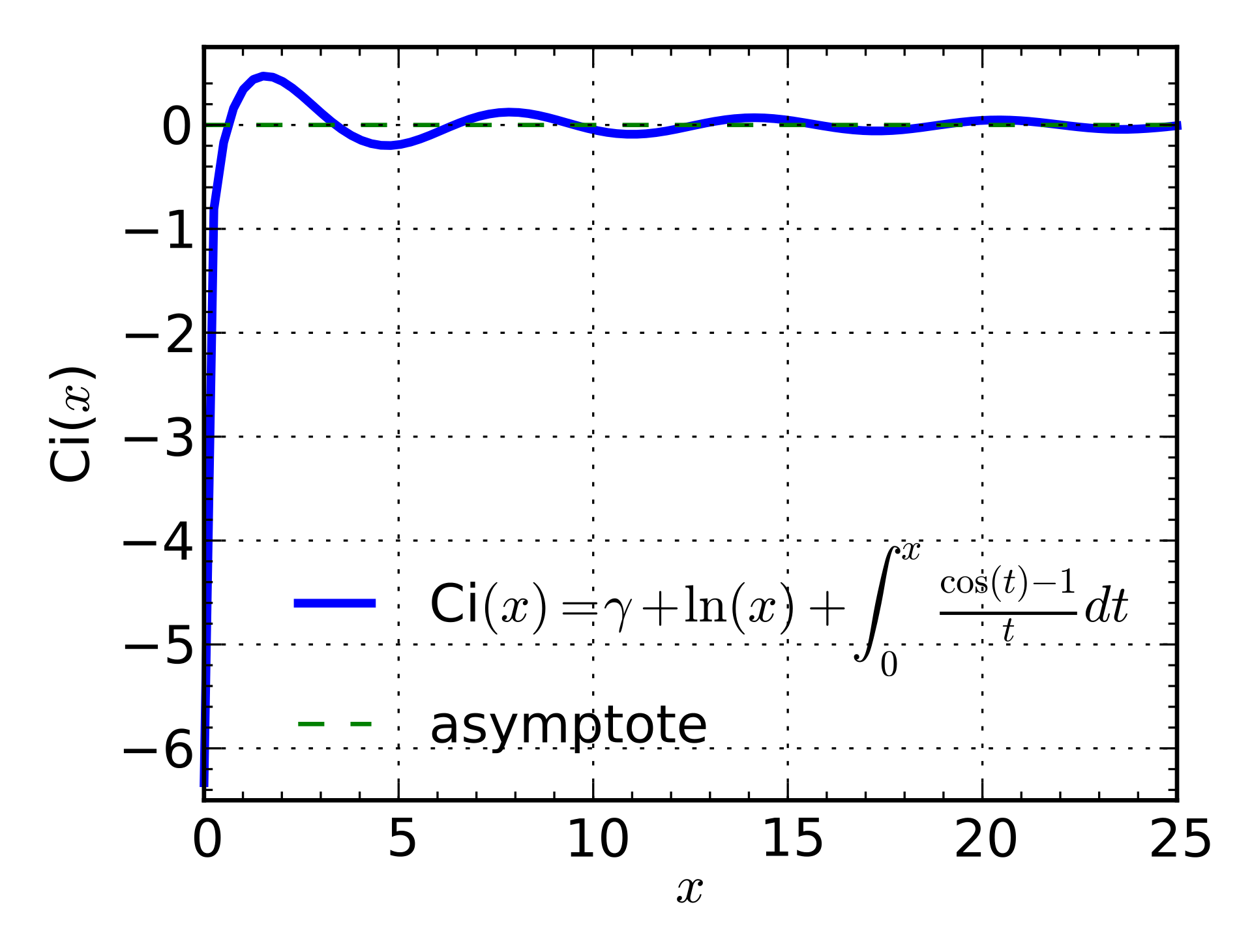[from Wikipedia" loading="lazy" referrerpolicy="no-referrer">Graph of Ci(x) [from Wikipedia]

Its first zero is at $x_0=0.6165\cdots$, and for $m\geq 1$, we can see that $|\text{Ci}(m)|\leq 1/2$, so $\text{Ci}(m)$ is actually a relatively small term and can be ignored for asymptotic estimation purposes. The problem then approximately reduces to requiring $\text{Ci}(mb^{-1})\leq 0$ to hold for all $m=1,2,\cdots,L$. This can be achieved simply by ensuring the corresponding $mb^{-1}$ all fall within the $[0,x_0]$ interval, which means $Lb^{-1}\leq x_0$, i.e.,

\begin{equation}b \geq L / x_0 \approx 2L\end{equation}

or more simply, $b^* = \mathcal{O}(L)$. As expected, this result is smaller than the exact numerical result, because it corresponds to $d\to\infty$: superimposing infinitely many trigonometric functions makes the resulting function oscillate less and appear smoother (compared to a finite $d$), so that for a fixed $b$, the continuous non-negative interval of $f_b(m)$ is longer — or conversely, for a fixed $L$, the smallest $b$ needed to keep $f_b(m)$ of $m=0,1,2,\cdots,L-1$ non-negative is smaller.

Related Thoughts

In Transformer Upgrade Path: 10. RoPE as a β-ary Encoding, we drew an analogy between RoPE and a base-$\beta$ representation, where $\beta = b^{2/d}$, so that $b - 1= \beta^{d/2} - 1$ is exactly the largest number representable by $d/2$ digits in base-$\beta$ notation. Thus, to represent $0,1,2,\cdots,L-1$ such positional encodings, we need at least $L$, giving us $b \geq L$. This simple analogy again leads to the conclusion that "$b$ should increase as $L$ increases," and its result is even closer to the asymptotic analysis result from the previous section.

On the other hand, Meta's newly released LLAMA3, with a training length of 8192, chose a surprisingly large RoPE base of 500000 (5e5) — nearly an order of magnitude larger than the earlier numerical result (8.4e4). No matter how you look at it, I think this value is on the large side; perhaps LLAMA3's base was already set with an eye toward an even larger context length. Regardless, it does seem to have become a common practice among many practitioners to choose a larger RoPE base for a larger text length.

In fact, whether via numerical results or asymptotic estimates, we only get a reference value. In practice, for a given $L$, a fairly wide range of $b$ values should give similar results. So the specific numbers aren't really what matters — the key contribution, in my view, is that the original paper starts from the idea of semantic aggregation and, through a series of derivations, clarifies the conclusion that "$b$ should increase as $L$ increases," along with its underlying reasoning. That is what I consider to be the core contribution of the paper.

Additionally, the starting point and conclusion of semantic aggregation can also be used to explain Position Interpolation (PI). As we just discussed, for a fixed $b$, the continuous non-negative interval of $f_b(m)$ is fixed. If we want $0,1,2,\cdots,L-1$ to all fall within the non-negative interval, we need to increase $b$ correspondingly as $L$ increases. But conversely, instead of increasing $b$, we could reduce the spacing between adjacent positions (i.e., change the position IDs to $0,1/k,2/k,\cdots$), which would allow us to represent $k$ times as many positions within the same-sized non-negative interval — this is Position Interpolation from the perspective of semantic aggregation.

Partial Rotation

RoPE was proposed in 2021, when there was only a single Chinese-language blog post about it. It was later recognized and experimented with by the EleutherAI organization, and only after that did it gradually spread within academia. At the time, EleutherAI's experiments found that applying RoPE to only part of the dimensions yielded slightly better results — related discussion can be found here, here, and here. This operation was later used in their GPT-NeoX.

Of course, partial rotation is still not the mainstream choice among current LLMs, but that shouldn't stop us from studying it — perhaps it hasn't become mainstream simply because we don't yet understand it well enough. So why might partial rotation actually be better? I've found that the conclusions of this article can, to some extent, explain it. Taking rotating only half the dimensions as an example, this is mathematically equivalent to choosing the following $\theta_i$:

\begin{equation}\theta_i = \left\{\begin{aligned}&b^{-4i/d},& i < d/4 \\ &0,&i \geq d/4\end{aligned}\right.\end{equation}

In this case, we have

\begin{equation}\sum_{i=0}^{d/2-1} \cos m\theta_i = \sum_{i=0}^{d/4-1} (1+\cos mb^{-4i/d})\geq 0\end{equation}

That is, regardless of what $m,b$ is, our desired inequality $\eqref{neq:base}$ automatically holds. This means that, from the perspective of this article, partial rotation provides positional information while achieving better semantic aggregation capability, which may well be more favorable for model performance. At the same time, partial rotation may also be more favorable for the model's long-text capability, because since the inequality holds unconditionally, according to the view presented here, there's no need to modify $b$ regardless of whether training is on short or long texts.

It's worth noting that the MLA proposed by DeepSeek also employs partial rotation, MLA. Although in MLA's original derivation, partial rotation was more of a necessary compromise for integrating RoPE, in light of previous experimental results on partial rotation, it's possible that MLA's excellent performance owes some credit to partial rotation as well.

Summary

This article gave a brief introduction to the paper Base of RoPE Bounds Context Length, which discusses the lower bound of RoPE's base from the perspective of the desired semantic-aggregation property, and points out that a larger training length should call for a larger base — not merely as a compromise for pairing with the "short-then-long" training strategy and using NTK-RoPE to lower the initial loss.