Variational Autoencoders (I): So That's What It's About

变分自编码器（一）：原来是这么一回事 苏剑林 · 2018-03-18 · Machine Learning variational unsupervised VAE generative model

I never studied it carefully before, but I've always had the impression that the Variational Auto-Encoder (VAE) was a good thing. So, riding the three-minutes-of-enthusiasm wave from recently reading about probabilistic graphical models, I decided to finally try to understand VAEs properly. As usual, I combed through a lot of material online, and without exception found it all rather vague — the general feeling was that a lot of formulas got written down, but things still felt murky. Even after I finally thought I'd understood it, when I went to look at implementation code, it felt like the code had nothing to do with the theory at all.

In the end, by piecing things together and drawing on some of the accumulated understanding of probabilistic models I've built up recently, and repeatedly comparing against the original paper Auto-Encoding Variational Bayes, I think I've finally figured it out. It turns out the real VAE is quite different from what many tutorials describe — a lot of them go on and on without ever really nailing down the key point of the model. So I wrote this piece, hoping the following text can give an initial, clear explanation of VAEs.

Distribution Transformation

We often compare VAEs to GANs, and indeed, their goals are essentially the same — to build a model that generates target data $X$ from a latent variable $Z$ — but they differ in implementation. More precisely, both assume that $Z$ follows some common distribution (such as a normal or uniform distribution), and then hope to train a model $X=g(Z)$ that maps this original probability distribution to the probability distribution of the training set. In other words, their goal in both cases is to perform a transformation between distributions.

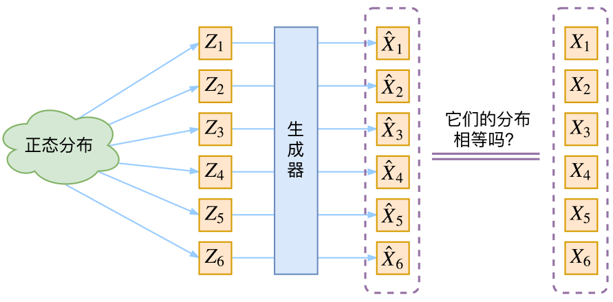The difficulty with generative models is judging the similarity between the generated distribution and the real distribution, because we only know the sampling results of the two, not their distribution expressions

Now suppose $Z$ follows a standard normal distribution. Then I can sample several $Z_1, Z_2, \dots, Z_n$ from it, transform them to get $\hat{X}_1 = g(Z_1),\hat{X}_2 = g(Z_2),\dots,\hat{X}_n = g(Z_n)$, and ask: how do we judge whether the dataset constructed via $g$ has the same distribution as our target dataset? Some readers might say, isn't there KL divergence for this? Of course that doesn't work directly, because KL divergence is computed from the expressions of two probability distributions, yet we don't actually know the expressions of these distributions — we only have a batch of data $\{\hat{X}_1,\hat{X}_2,\dots,\hat{X}_n\}$ sampled from the constructed distribution, and a batch of data $\{X_1,X_2,\dots,X_n\}$ sampled from the real distribution (i.e., the training set we want to generate). We only have the samples themselves, not the distribution expressions, so of course there's no way to compute the KL divergence.

Even though we've hit an obstacle, we still need to find a way forward. GAN's approach is direct and brute-force: since there's no suitable metric, why not just train the metric itself with a neural network? That's how WGAN came about — for the details, see The Art of Mutual Sabotage: Getting Straight to WGAN-GP. VAE, on the other hand, uses a more delicate, roundabout trick.

A Leisurely Chat About VAE

Let's first review how VAE is typically introduced in tutorials, then investigate what's problematic about that account, and from there we'll naturally uncover the true face of VAE.

The Classic Account

First, we have a batch of data samples $\{X_1,\dots,X_n\}$, whose overall distribution we describe with $X$. What we'd really like is to obtain the distribution of $X$, i.e., $p(X)$, directly from $\{X_1,\dots,X_n\}$. If we could get that, we could simply sample according to $p(X)$ to obtain every possible $X$ (including ones beyond $\{X_1,\dots,X_n\}$) — this would be the ultimate ideal generative model. Of course, this ideal is hard to achieve, so we rewrite the distribution as

$$p(X)=\sum_Z p(X|Z)p(Z)\tag{1}$$

Here we won't bother distinguishing sums from integrals — the meaning is what matters. Now $p(X|Z)$ describes a model that generates $X$ from $Z$, and we assume $Z$ follows a standard normal distribution, i.e., $p(Z)=\mathcal{N}(0,I)$. If this ideal could be realized, then we could first sample a $Z$ from the standard normal distribution, then compute a $X$ according to $Z$ — also a rather nice generative model. Next comes combining this with autoencoders to achieve reconstruction, ensuring no useful information is lost, and after a bunch of further derivation, finally implementing the model. A schematic diagram of this framework looks like this:

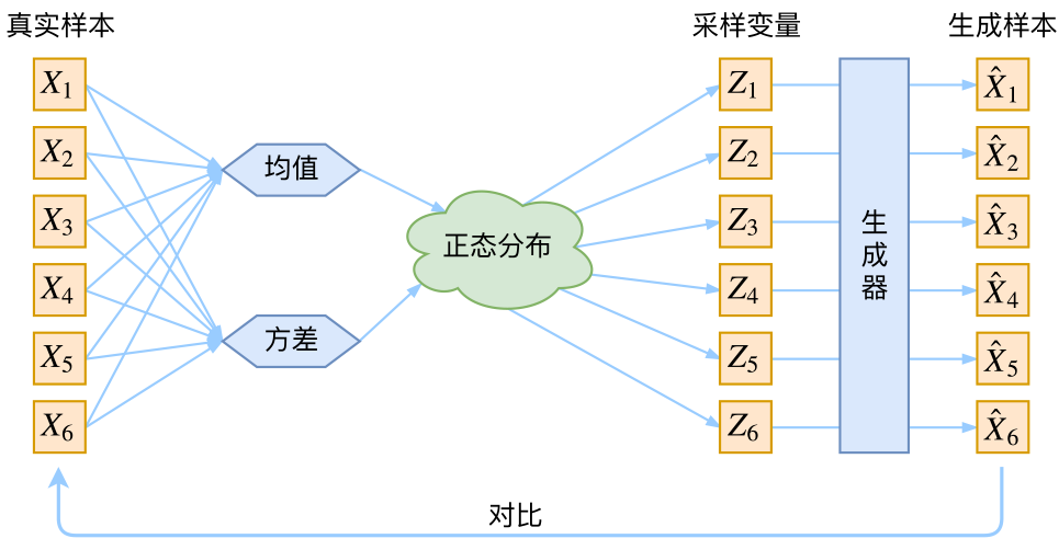The conventional understanding of VAE

Do you see the problem here? Going by this diagram, we actually have no idea whether the resampled $Z_k$ still corresponds to the original $X_k$. So directly minimizing $\mathcal{D}(\hat{X}_k,X_k)^2$ (where $\mathcal{D}$ denotes some distance function) is not well-founded at all — and indeed, if you look at the code, you'll find it's implemented quite differently from this. In other words, a lot of tutorials talk a big and seemingly coherent game, but then write code that doesn't match what they said — and somehow they don't find this contradictory at all.

VAE Revealed

In fact, nowhere in the actual VAE model do we use the assumption that $p(Z)$ (the distribution over the latent variable space) is normal. What we actually assume is that $p(Z|X)$ (the posterior distribution) is normal!!

Specifically, given a real sample $X_k$, we assume there exists a distribution $p(Z|X_k)$ specific to $X_k$ (formally called the posterior distribution), and we further assume this distribution is (independent, multivariate) normal. Why emphasize "specific to"? Because later we'll train a generator $X=g(Z)$ that is meant to map a $Z_k$ sampled from the distribution $p(Z|X_k)$ back to $X_k$. If we instead assumed $p(Z)$ was normal and sampled a $Z$ from $p(Z)$, how would we know which real $X$ this $Z$ corresponds to? Now that $p(Z|X_k)$ is specific to $X_k$, we have good reason to say that a $Z$ sampled from this distribution ought to be reconstructed back into $X_k$.

Indeed, in the application section of the paper Auto-Encoding Variational Bayes, this point is specifically emphasized:

In this case, we can let the
variational approximate posterior be a multivariate Gaussian with a diagonal covariance structure:
$$\log q_{\phi}(\boldsymbol{z}|\boldsymbol{x}^{(i)}) = \log \mathcal{N}(\boldsymbol{z} ;\boldsymbol{\mu}^{(i)},\boldsymbol{\sigma}^{2(i)}\boldsymbol{I})\tag{9}$$
(Note: this is quoted directly from the original paper; the notation used in this article doesn't exactly match the original paper's, but hopefully readers won't be confused.)

Equation $(9)$ in the paper is the key to implementing the whole model, and I'm not sure why so many tutorials fail to highlight it when introducing VAE. Although the paper also mentions that $p(Z)$ is a standard normal distribution, that's actually not the essential point.

Back to our discussion: at this point every $X_k$ has been given its own dedicated normal distribution, which makes it much easier for the generator to reconstruct it later. But that means there are as many normal distributions as there are $X$'s. We know a normal distribution has two sets of parameters: mean $\mu$ and variance $\sigma^2$ (both vectors, in the multivariate case), so how do we find the mean and variance of the distribution $p(Z|X_k)$ specific to $X_k$? There's no obvious direct way. Well then — let's just fit them with a neural network! This is the philosophy of the neural-network era: whatever's hard to compute exactly, we fit with a neural network; we already saw this once with WGAN, and now we're seeing it again.

So we build two neural networks $\mu_k = f_1(X_k),\log \sigma_k^2 = f_2(X_k)$ to compute these quantities. We choose to fit $\log \sigma_k^2$ rather than directly fitting $\sigma_k^2$, because $\sigma_k^2$ is always non-negative and would require an activation function, whereas fitting $\log \sigma_k^2$ requires no activation function since it can be positive or negative. At this point, we know the mean and variance specific to $X_k$, so we know exactly what its dedicated normal distribution looks like. We then sample a $Z_k$ from this dedicated distribution, pass it through a generator to get $\hat{X}_k=g(Z_k)$, and now we can confidently minimize $\mathcal{D}(\hat{X}_k,X_k)^2$, because $Z_k$ was sampled from the distribution specific to $X_k$, and this generator should be able to reconstruct the original $X_k$ from it. So we can draw the VAE schematic as follows:

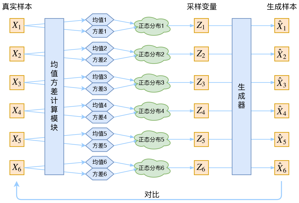In fact, VAE constructs a dedicated normal distribution for each sample and then samples from it to reconstruct

Standardizing the Distribution

Let's think about what result this training process, as depicted above, would ultimately produce.

First, we want to reconstruct $X$, i.e., minimize $\mathcal{D}(\hat{X}_k,X_k)^2$, but this reconstruction process is affected by noise, because $Z_k$ has been resampled and is not computed directly by the encoder. Clearly noise makes reconstruction harder — but fortunately, this noise's intensity (i.e., the variance) is computed by a neural network, so ultimately, in order to reconstruct better, the model will try its best to drive the variance to zero. And once the variance is zero, there's no more randomness — no matter how you sample, you'll always get the same deterministic result (namely the mean); and of course fitting just one value is easier than fitting many, and the mean is computed by another neural network.

Put simply, the model would gradually degenerate into an ordinary AutoEncoder, and the noise would stop playing any role.

Wouldn't that be a wasted effort? What happened to the generative model we were promised?

Don't worry — in fact, VAE also pushes all the $p(Z|X)$ distributions toward the standard normal distribution, which prevents the noise from vanishing to zero, while at the same time guaranteeing that the model has generative capability. How should we understand "guaranteeing generative capability"? If all the $p(Z|X)$ are close to the standard normal distribution $\mathcal{N}(0,I)$, then by definition

$$p(Z)=\sum_X p(Z|X)p(X)=\sum_X \mathcal{N}(0,I)p(X)=\mathcal{N}(0,I) \sum_X p(X) = \mathcal{N}(0,I)\tag{2}$$

This lets us achieve our prior assumption: that $p(Z)$ is a standard normal distribution. Then we can confidently sample from $\mathcal{N}(0,I)$ to generate images.

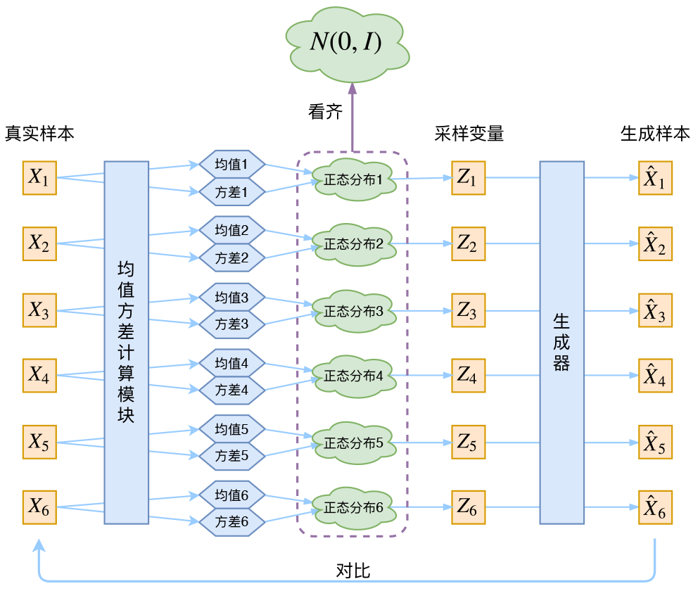To give the model generative capability, VAE requires every p(Z_X) to align with the normal distribution

So how do we push all the $p(Z|X)$'s toward $\mathcal{N}(0,I)$? Without any external knowledge, the most direct approach would probably be to add an extra loss on top of the reconstruction error:

$$\mathcal{L}_{\mu}=\Vert f_1(X_k)\Vert^2\quad \text{and}\quad \mathcal{L}_{\sigma^2}=\Vert f_2(X_k)\Vert^2\tag{3}$$

since these terms represent the mean $\mu_k$ and the log variance $\log\sigma_k^2$ respectively, and reaching $\mathcal{N}(0,I)$ means we want both to approach 0. However, this raises the question of how to choose the relative weighting between these two losses — if chosen poorly, the generated images tend to come out blurry. So instead, the original paper directly computes the KL divergence $KL\Big(N(\mu,\sigma^2)\Big\Vert N(0,I)\Big)$ between the general (component-wise independent) normal distribution and the standard normal distribution, and uses this as the extra loss, giving

$$\mathcal{L}_{\mu,\sigma^2}=\frac{1}{2} \sum_{i=1}^d \Big(\mu_{(i)}^2 + \sigma_{(i)}^2 - \log \sigma_{(i)}^2 - 1\Big)\tag{4}$$

Here $d$ is the dimensionality of the latent variable $Z$, and $\mu_{(i)}$ and $\sigma_{(i)}^2$ denote the $i$-th components of the mean vector and variance vector of the general normal distribution, respectively. Using this expression directly as the auxiliary loss sidesteps the problem of weighting mean loss against variance loss. Clearly, this loss can also be understood as two parts:

$$\begin{aligned}&\mathcal{L}_{\mu,\sigma^2}=\mathcal{L}_{\mu} + \mathcal{L}_{\sigma^2}\\ &\mathcal{L}_{\mu}=\frac{1}{2} \sum_{i=1}^d \mu_{(i)}^2=\frac{1}{2}\Vert f_1(X)\Vert^2\\ &\mathcal{L}_{\sigma^2}=\frac{1}{2} \sum_{i=1}^d\Big(\sigma_{(i)}^2 - \log \sigma_{(i)}^2 - 1\Big)\end{aligned}\tag{5}$$

Derivation
Since we're dealing with a multivariate normal distribution with independent components, it suffices to derive the univariate normal case. By definition, we can write
$$\begin{aligned}&KL\Big(N(\mu,\sigma^2)\Big\Vert N(0,1)\Big)\\ > =&\int \frac{1}{\sqrt{2\pi\sigma^2}}e^{-(x-\mu)^2/2\sigma^2} \left(\log \frac{e^{-(x-\mu)^2/2\sigma^2}/\sqrt{2\pi\sigma^2}}{e^{-x^2/2}/\sqrt{2\pi}}\right)dx\\ > =&\int \frac{1}{\sqrt{2\pi\sigma^2}}e^{-(x-\mu)^2/2\sigma^2} \log \left\{\frac{1}{\sqrt{\sigma^2}}\exp\left\{\frac{1}{2}\big[x^2-(x-\mu)^2/\sigma^2\big]\right\} \right\}dx\\ > =&\frac{1}{2}\int \frac{1}{\sqrt{2\pi\sigma^2}}e^{-(x-\mu)^2/2\sigma^2} \Big[-\log \sigma^2+x^2-(x-\mu)^2/\sigma^2 \Big] dx\end{aligned}$$
The result splits into three integral terms. The first is essentially $-\log \sigma^2$ times the integral of the probability density (which equals 1), so it equals $-\log \sigma^2$; the second term is actually the second moment of the normal distribution, and anyone familiar with the normal distribution will know its second moment equals $\mu^2+\sigma^2$; and by definition, the third term is simply "minus the variance divided by the variance = -1." So the overall result is $$KL\Big(N(\mu,\sigma^2)\Big\Vert N(0,1)\Big)=\frac{1}{2}\Big(-\log \sigma^2+\mu^2+\sigma^2-1\Big)$$

The Reparameterization Trick

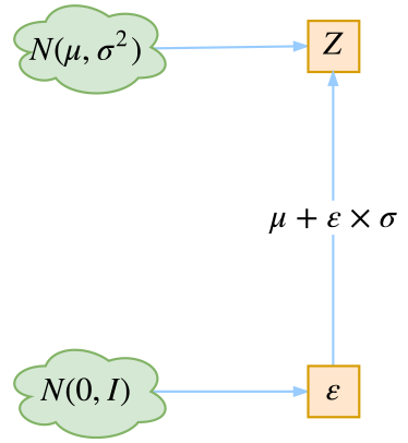The reparameterization trick

Last but not least is a trick used to actually implement the model — the English name is "reparameterization trick," which I'll just call "reparameterization" here. It's actually quite simple. We need to sample a $Z_k$ from $p(Z|X_k)$; although we know $p(Z|X_k)$ is normal, with the mean and variance computed by a model, and we need this sampling process in order to backpropagate and optimize the mean/variance networks — the "sampling" operation itself is not differentiable, but the result of sampling is. We use the fact that

$$\begin{aligned}&\frac{1}{\sqrt{2\pi\sigma^2}}\exp\left(-\frac{(z-\mu)^2}{2\sigma^2}\right)dz \\ =& \frac{1}{\sqrt{2\pi}}\exp\left[-\frac{1}{2}\left(\frac{z-\mu}{\sigma}\right)^2\right]d\left(\frac{z-\mu}{\sigma}\right)\end{aligned}\tag{6}$$

which shows that $(z-\mu)/\sigma=\varepsilon$ follows a standard normal distribution with mean 0 and variance 1. We need to include $dz$ as well, since multiplying by $dz$ is what turns this into an actual probability — dropping $dz$ leaves us with a probability density, not a probability. This gives us:

Sampling a $Z$ from $\mathcal{N}(\mu,\sigma^2)$ is equivalent to sampling a $\varepsilon$ from $\mathcal{N}(0,I)$, and then letting $Z=\mu + \varepsilon \times \sigma$.

So we've turned sampling from $\mathcal{N}(\mu,\sigma^2)$ into sampling from $\mathcal{N}(0,I)$, followed by a parameter transformation to get the result of sampling from $\mathcal{N}(\mu,\sigma^2)$. This way, the "sampling" operation itself no longer needs to be part of gradient descent — instead, the result of sampling participates, which makes the whole model trainable.

As for exactly how this is implemented, just match up the above text against the code and it'll click right away.

Further Analysis

Even with everything above cleared up, we might still have plenty of lingering questions about VAE.

What Is the Essence of It?

What is the essence of VAE? While VAE is also called a kind of AE (AutoEncoder), its approach (or rather, its interpretation of the network) is quite distinctive. In VAE, there are two encoders: one computes the mean, and the other computes the variance. This alone is already surprising: the "encoder" isn't encoding at all — it's computing means and variances! And aren't the mean and variance supposed to be statistics? How can they be computed by a neural network?

In fact, I think that although VAE starts from variational calculus and Bayesian theory — subjects that intimidate the average person — and takes a fairly long road to arrive at a concrete model, the final model is actually quite down-to-earth: it's essentially a regular autoencoder, where "Gaussian noise" has been added to the output of the encoder (in VAE, this corresponds to the network computing the mean), so that the decoder is made robust to this noise; and the extra KL loss (whose purpose is to push the mean toward 0 and the variance toward 1) is, in effect, a regularization term on the encoder, encouraging the encoder's output to have zero mean.

So what's the role of the other encoder (the one computing the variance)? It dynamically adjusts the strength of the noise. Intuitively, when the decoder hasn't been trained well yet (reconstruction error much larger than the KL loss), the noise is appropriately reduced (KL loss increases), making the fitting task easier (reconstruction error starts to drop); conversely, once the decoder has been trained reasonably well (reconstruction error smaller than the KL loss), the noise increases (KL loss decreases), making the fitting task harder again (reconstruction error starts rising again), at which point the decoder has to find a way to boost its generative power.

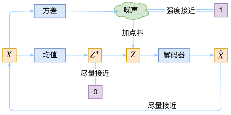The essential structure of VAE

In short, the reconstruction process wants there to be no noise, while the KL loss wants there to be Gaussian noise — the two are in opposition. So, just like GAN, VAE internally contains an adversarial process, except here the two sides are blended together and co-evolve. From this angle, VAE's idea might even seem cleverer, because in GAN, while the forger is evolving, the discriminator sits still, and vice versa. Of course, this is only one facet — it doesn't mean VAE is better than GAN. What's truly clever about GAN is that it learns the metric itself directly, and this learned metric is often better than anything we could design by hand (though GAN itself has plenty of its own issues, which we won't get into here).

From this discussion, we can also see that, naturally, no individual $p(Z|X)$ can be exactly equal to the standard normal distribution — otherwise $p(Z|X)$ would become completely independent of $X$, and reconstruction would be terrible. What ends up happening instead is that $p(Z|X)$ retains a certain amount of information about $X$, giving reasonably good reconstruction, while $(2)$ approximately holds, thereby preserving generative capability at the same time.

Does It Have to Be Normal?

Regarding the distribution of $p(Z|X)$, readers might wonder: does it have to be a normal distribution? Could we use a uniform distribution instead?

Probably not very feasible — and this again comes down to the formula for KL divergence:

$$KL\Big(p(x)\Big\Vert q(x)\Big) = \int p(x) \ln \frac{p(x)}{q(x)}dx\tag{7}$$

If there's some region where $p(x)\neq 0$ while $q(x)=0$, then the KL divergence blows up to infinity. For the normal distribution, the probability density is positive everywhere, so this issue never arises. But for the uniform distribution, as long as the two distributions don't coincide exactly, there will inevitably be some interval where $p(x)\neq 0$ while $q(x)=0$, causing the KL divergence to diverge. Of course, when writing code we'd guard against such division-by-zero errors, but we still can't avoid the KL loss dominating disproportionately, causing the model to rapidly drive the KL loss down — meaning the posterior distribution $p(Z|X)$ collapses quickly toward the prior $p(Z)$, and the noise and reconstruction can no longer play their adversarial roles against each other. This brings us right back to where we started: we'd be unable to tell which $z$ corresponds to which $x$.

Of course, insisting on a uniform distribution isn't strictly impossible — you'd just need to work out the KL divergence between two uniform distributions, carefully handle division-by-zero errors, increase the weight on the reconstruction loss, and so on. But it would end up looking rather ugly.

Where's the "Variational" Part?

Here's another interesting (though not terribly important) question: VAE stands for "Variational Auto-Encoder" — what does it actually have to do with variational calculus? In VAE papers and related explanations, we don't seem to see variational calculus showing up anywhere.

Well — actually, if you've already accepted KL divergence as a given, then VAE really doesn't seem to have much to do with variational calculus after all. That's because, in theory, for the KL divergence $(7)$ we need to prove:

Fixing the probability distribution $p(x)$ (or $q(x)$), for any probability distribution $q(x)$ (or $p(x)$), we have $KL\Big(p(x)\Big\Vert q(x)\Big)\geq 0$, with equality holding only when $p(x)=q(x)$.

Because $KL\Big(p(x)\Big\Vert q(x)\Big)$ is actually a functional, finding the extremum of a functional requires the calculus of variations. Of course, the variational calculus used here is just a straightforward parallel extension of ordinary calculus, not yet touching on the genuinely complex machinery of variational calculus. And VAE's variational lower bound is derived directly from the KL divergence. So once you've accepted the KL divergence as given, there's really no more work for "variational calculus" to do.

In a nutshell, the "variational" in VAE's name refers to the fact that its derivation makes use of the KL divergence and its properties.

Conditional VAE

Finally, since the current VAE is trained in an unsupervised manner, it's natural to wonder: if we have labeled data, can we incorporate the label information to help guide sample generation? The motivation behind this question is usually the hope of being able to control some variable so as to generate a specific class of images. This is certainly possible — we call this scenario a Conditional VAE, or CVAE. (Correspondingly, in GAN we also have a CGAN.)

But CVAE isn't a single specific model — it's a whole family of models; there are many ways of folding label information into VAE, serving different purposes. Here, building on the earlier discussion, I'll give a very simple version of a CVAE.

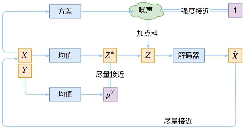The structure of a simple CVAE

In the earlier discussion, we wanted the distribution of $Z$ to have zero mean and unit variance after encoding $X$, and this "wish" was realized by adding the KL loss. Now if we additionally have class information $Y$, we can instead wish that samples from the same class share a dedicated mean $\mu^Y$ (keeping the variance unchanged at unit variance), letting the model learn this $\mu^Y$ on its own during training. In this way, there'd be as many normal distributions as there are classes, and at generation time we can control the class of the generated image by controlling the mean. In fact, this is likely the way of implementing CVAE that requires adding the least amount of code on top of VAE, since this "new wish" only requires modifying the KL loss:

$$\mathcal{L}_{\mu,\sigma^2}=\frac{1}{2} \sum_{i=1}^d\Big[\big(\mu_{(i)}-\mu^Y_{(i)}\big)^2 + \sigma_{(i)}^2 - \log \sigma_{(i)}^2 - 1\Big]\tag{8}$$

The figure below shows that this simple CVAE does have some effect, although since both the encoder and decoder here are fairly simple (pure MLPs), the control over generation isn't perfect. Readers interested in a more thorough CVAE are encouraged to study further on their own — there's also recent work combining CVAE with GAN, CVAE-GAN, since the landscape of model tricks keeps evolving in every direction.

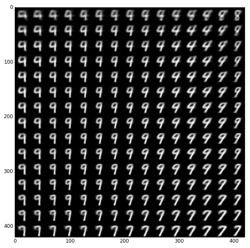Using this CVAE to control generation of the digit 9, we can see it produces multiple styles of 9, gradually transitioning toward 7, suggesting this CVAE is indeed effective on preliminary inspection

Code

I took Keras's official VAE code, made some tweaks, and added Chinese comments based on the content of this post; I've also implemented the simple CVAE described above, for readers' reference.

Code: https://github.com/bojone/vae

Terminus

Bumpy road, but we've reached the end of the article. I'm not sure whether I've explained things clearly — please feel free to offer feedback.

Overall, I think the idea behind VAE is really quite elegant. Not because it provides an especially great generative model (in fact its generated images aren't all that good — a bit blurry) — but because it provides a wonderful case study of combining probabilistic graphical models with deep learning, and this case has plenty worth pondering and savoring.