Fitting a One-Dimensional Probability Density Function with Fourier Series

用傅里叶级数拟合一维概率密度函数 苏剑林 · 2024-03-07 · Mathematics series probability analysis approximation

In Closed-Door Multimodal Musings (I): Lossless Input] we mentioned that the fundamental difficulty of image generation is the lack of a universal fitter for continuous probability densities. Of course, that's not entirely true — the Gaussian Mixture Model (GMM), for instance, is in theory capable of fitting any probability density, and even GANs can essentially be understood as a GMM with infinitely many mixed Gaussians. However, although GMM has sufficient theoretical capacity, maximum likelihood estimation with it is difficult, and in particular it generally doesn't lend itself to gradient-based optimizers, which limits its use cases.

Recently, a new paper from Google, Fourier Basis Density Model], proposed a new solution for the one-dimensional case — fitting with Fourier series. The paper's analysis is quite interesting and its construction is clever, well worth studying.

Problem Statement

Some readers might question: what's the value of studying only the one-dimensional case? Indeed, if we only consider image generation, the value might really be limited. But one-dimensional probability density estimation has its own applications, such as lossy data compression, so it remains a topic worth studying. Moreover, even if we need to study multi-dimensional probability densities, we can convert the problem into estimating multiple one-dimensional conditional probability densities via autoregression. Finally, this analysis and construction process is itself worth savoring, so even treating it purely as a mathematical exercise is quite beneficial. more

Back to the main topic. So-called one-dimensional probability density estimation refers to: given $n$ real numbers $x_1,x_2,\cdots,x_n$ sampled from the same distribution, estimate the probability density function of the sampling distribution. Methods for this problem fall into two categories: "non-parametric estimation" and "parametric estimation." Non-parametric estimation mainly refers to kernel density estimation, which, like in Using the Dirac Function to Construct Smooth Approximations of Non-Smooth Functions], essentially uses the Dirac function to make a smooth approximation:

\begin{equation}p(x) = \int p(y)\delta(x - y) = \mathbb{E}_{y\sim p(y)}[\delta(x - y)]\approx \frac{1}{n}\sum_{i=1}^n \delta(x - x_i)\label{eq:delta}\end{equation}

But $\delta(x - y)$ is not an ordinary smooth function, so we need to find a smooth approximation of it, such as $\frac{e^{-(x-y)^2/2\sigma^2}}{\sqrt{2\pi}\sigma}$, which is the probability density function of the normal distribution; when $\sigma\to 0$ it becomes $\delta(x-y)$. Substituting into the above equation gives us "Gaussian kernel density estimation."

We can see that kernel density estimation essentially just memorizes the data, so we'd expect it to have limited generalization ability. Additionally, its complexity is proportional to the amount of data, so it's impractical when the data scale is large. This is why we need "parametric estimation": constructing a family of non-negative, normalized probability density functions $p_{\theta}(x)$ with a fixed amount of parameters $\theta$, which can then be solved via maximum likelihood:

\begin{equation}\theta^* = \mathop{\text{argmax}}_{\theta} \sum_{i=1}^n \log p_{\theta}(x_i)\end{equation}

The key to this problem is how to construct a family of probability density functions $p_{\theta}(x)$ with sufficient fitting capacity.

Existing Methods

The classic method for parametric probability density estimation is the Gaussian Mixture Model (GMM). It also starts from equation $\eqref{eq:delta}$ plus a Gaussian kernel, but instead of iterating over all data points as centers, it finds a finite number of $K$ means and variances through training, constructing a model whose complexity is independent of the data size:

\begin{equation}p_{\theta}(x) = \frac{1}{K}\sum_{i=1}^K \frac{e^{-(x-\mu_i)^2/2\sigma_i^2}}{\sqrt{2\pi}\sigma_i},\quad \theta = \{\mu_1,\sigma_1,\mu_2,\sigma_2,\cdots,\mu_K,\sigma_K\}\end{equation}

GMM is often also understood as a clustering method — a generalization of K-Means, where $\mu_1,\mu_2,\cdots,\mu_K$ are the cluster centers, with the addition of variance $\sigma_1,\sigma_2,\cdots,\sigma_K$ compared to K-Means. Thanks to the theoretical guarantee of equation $\eqref{eq:delta}$, when $K$ is large enough and $\sigma$ is small enough, GMM can in theory always fit an arbitrarily complex distribution, so GMM's theoretical capacity is sufficient. But the problem with GMM is that the form $e^{-(x-\mu_i)^2/2\sigma_i^2}$ decays too quickly, causing severe vanishing gradients, so it's usually only solvable with the EM algorithm (see Three Flavors of Capsules: Matrix Capsules and EM Routing]) — it doesn't work well with gradient-based optimizers, which limits its applicability. And even with EM, one usually only finds a suboptimal solution.

The original paper also mentions a method called DFP (Deep Factorized Probability), designed specifically for one-dimensional probability density estimation, from the paper Variational Image Compression with a Scale Hyperprior]. DFP exploits the monotonicity of the cumulative distribution function, i.e. the following integral

\begin{equation}\Phi(x) = \int_{-\infty}^x p(y)dy \in [0,1]\end{equation}

must necessarily be monotonically increasing. If we can first construct a monotonically increasing function $\Phi_{\theta}(x)$ over $\mathbb{R}\mapsto[0,1]$, then differentiating it gives a valid probability density function. How do we ensure that a model's output is monotonically increasing with respect to its input? DFP builds the model with a multi-layer neural network, guaranteeing: 1) all activation functions are monotonically increasing; 2) all multiplicative weights are non-negative. Under these two constraints, the model necessarily has the monotonically-increasing property, and finally adding a sigmoid lets us control the range to be $[0,1]$.

The principle behind DFP is simple and intuitive, but similar to flow-based models, this kind of layer-by-layer constraint raises concerns about losing fitting capacity. Moreover, since this model is entirely built from a neural network, based on previous results such as Frequency Principle: Fourier Analysis Sheds Light on Deep Neural Networks], neural networks tend to learn low-frequency signals preferentially during training, which may cause DFP to fit peak points of the probability density poorly — that is, produce an overly smoothed fit. Yet in many scenarios, the ability to fit peaks is one of the important metrics for evaluating a probabilistic modeling method.

Enter Fourier

As the paper's title, "Fourier Basis Density Model" (abbreviated below as FBDM), suggests, the new method proposed in the paper fits the probability density based on Fourier series. To be fair, it's not that hard to think of using Fourier series for fitting — what's hard is that there's a key non-negativity constraint that's not easy to construct, and FBDM works out all the relevant details, which is quite admirable.

For simplicity, let's set the domain of $x$ to be $[-1,1]$. Since we can always compress any real numbers on $\mathbb{R}$ down to $[-1,1]$ via a transformation like $\tanh$, this setup loses no generality. That is, the probability density function $p(x)$ we're now seeking is a function defined on $[-1,1]$, so we can write it as a Fourier series

\begin{equation}p(x) = \sum_{n=-\infty}^{\infty} c_n e^{i\pi n x},\quad c_n = \frac{1}{2}\int_{-1}^1 p(x) e^{-i\pi n x} dx\end{equation}

However, what we now want to do is the reverse: rather than knowing $p(x)$ and computing its Fourier series, we only know samples of $p(x)$, and we need to set $p(x)$ to the following truncated Fourier series form, then solve for the coefficients $c_n$ using an optimizer:

\begin{equation}f_{\theta}(x) = \sum_{n=-N}^{N} c_n e^{i\pi n x},\quad \theta = \{c_{-N},c_{-N+1},\cdots,c_{N-1},c_N\}\label{eq:fourier-series}\end{equation}

As we all know, for $f_{\theta}(x)$ to be a valid probability density function, it must at least satisfy the following two conditions:

\begin{equation}\text{non-negative:}\,\,f_{\theta}(x)\geq 0,\quad \text{normalize:}\,\,\int_{-1}^1 f_{\theta}(x)dx = 1\end{equation}

The problem is that if $c_n$ takes arbitrary real/complex values, then it's not even guaranteed that equation $\eqref{eq:fourier-series}$ is real-valued, let alone non-negative. So, using Fourier series for fitting isn't hard to think of — the hard part is how to set the form of $c_n$ so that the corresponding output is necessarily non-negative (as we'll see later, under Fourier series, the hardest part is non-negativity — normalization, by contrast, is easy).

Ensuring Non-Negativity

In this section we'll look at the most difficult construction in the whole paper: non-negativity. Of course, the difficulty here isn't that the derivation is especially complex, but rather that it's very clever.

First, we know that being non-negative presupposes being real-valued, and ensuring real-valuedness is relatively simple:

\begin{equation}c_n^* = \left[\frac{1}{2}\int_{-1}^1 p(x) e^{-i\pi n x} dx\right]^* = \frac{1}{2}\int_{-1}^1 p(x) e^{i\pi n x} dx = c_{-n}\end{equation}

Conversely, one can prove that this condition is also sufficient, so ensuring realness only requires constraining $c_n^* = c_{-n}$, which is relatively easy to achieve; this also means that when the series in equation $\eqref{eq:fourier-series}$ serves as a probability density function, there are only $N+1$ independent parameters, $c_0,c_1,\cdots,c_N$.

Regarding the non-negativity constraint, the original paper simply cites "Herglotz's theorem" and then directly gives the answer, with almost no derivation. The author searched for Herglotz's theorem and found few introductions to it, so I'll try to skip Herglotz's theorem and understand the original paper's answer in my own way.

Consider any finite subset of integers $\mathbb{K}\subseteq\mathbb{N}$, and a corresponding arbitrary sequence of complex numbers $\{u_k|k\in\mathbb{K}\}$. We have

\begin{equation}\begin{aligned} \sum_{n,m\in \mathbb{K}} u_n^* c_{n-m} u_m =&\, \sum_{n,m\in \mathbb{K}} u_n^* \left[\frac{1}{2}\int_{-1}^1 p(x) e^{-i\pi (n-m) x} dx\right] u_m \\ =&\, \frac{1}{2}\int_{-1}^1 p(x) \left[\sum_{n,m\in \mathbb{K}} u_n^* e^{-i\pi (n-m) x} u_m \right] dx \\ =&\, \frac{1}{2}\int_{-1}^1 p(x) \sum_{n,m\in \mathbb{K}} \left[(u_n e^{i\pi n})^* (u_m e^{i\pi m})\right] dx \\ =&\, \frac{1}{2}\int_{-1}^1 p(x) \left[\left(\sum_{n\in \mathbb{K}}u_n e^{i\pi n}\right)^* \left(\sum_{m\in \mathbb{K}}u_m e^{i\pi m}\right)\right] dx \\ =&\, \frac{1}{2}\int_{-1}^1 p(x) \left|\sum_{n\in \mathbb{K}}u_n e^{i\pi n}\right|^2 dx \\ \geq&\, 0 \\ \end{aligned}\end{equation}

The final $\geq 0$ depends on $p(x)\geq 0$, so we obtain a necessary condition for $f_{\theta}(x)\geq 0$: $\sum\limits_{n,m\in \mathbb{K}} u_n^* c_{n-m} u_m\geq 0$. If we arrange all $c_{n-m}$ into one large matrix (a Toeplitz matrix), then in the language of linear algebra, this condition says that the submatrix formed by the row-and-column intersections corresponding to any $\mathbb{K}$ must be a positive-definite matrix over complex space. One can also prove that this condition is sufficient, i.e. any $f_{\theta}(x)$ satisfying this condition is necessarily always greater than 0.

So the problem becomes: how do we find a sequence of complex numbers $\{c_n\}$ such that the corresponding Toeplitz matrix $\{c_{n-m}\}$ is positive definite? This seems to make the problem even more complicated, but readers familiar with time series may already know a ready-made construction: the "autocorrelation coefficient]." For an arbitrary sequence of complex numbers $\{a_k\}$, the autocorrelation coefficient is defined as

\begin{equation}r_n = \sum_{k=-\infty}^{\infty} a_k a_{k+n}^*\end{equation}

One can prove that $r_{n-m}$ is necessarily positive definite:

\begin{equation}\begin{aligned} \sum_{n,m\in \mathbb{K}} u_n^* r_{n-m} u_m =&\, \sum_{n,m\in \mathbb{K}} u_n^* \left(\sum_{k=-\infty}^{\infty} a_k a_{k+n-m}^*\right) u_m \\ =&\, \sum_{n,m\in \mathbb{K}} u_n^* \left(\sum_{k=-\infty}^{\infty} a_{k+m} a_{k+n}^*\right) u_m \\ =&\, \sum_{k=-\infty}^{\infty}\left(\sum_{n\in \mathbb{K}} a_{k+n} u_n\right)^*\left(\sum_{m\in \mathbb{K}} a_{k+m} u_m\right) \\ =&\, \sum_{k=-\infty}^{\infty}\left|\sum_{n\in \mathbb{K}} a_{k+n} u_n\right|^2 \\ \geq&\, 0 \end{aligned}\end{equation}

Therefore, taking $c_n$ to be of the form $r_n$ is a viable solution. To ensure that $c_n$ has only $N+1$ independent parameters, we stipulate that $a_k=0$ when $k < 0$ or $k > N$, giving

\begin{equation}c_n = \sum_{k=0}^{N-n} a_k a_{k+n}^*\end{equation}

This constructs the corresponding $c_n$, ensuring that the result of the Fourier series in equation $\eqref{eq:fourier-series}$ is necessarily non-negative, satisfying the non-negativity requirement of a probability density function.

The General Result

At this point, the hardest part of the whole problem — "non-negativity" — has been solved. The remaining normalization is simple, because

\begin{equation}\int_{-1}^1 f_{\theta}(x)dx = \int_{-1}^1 \sum_{n=-N}^{N} c_n e^{i\pi n x} dx = 2c_0\end{equation}

so the normalization factor is simply $2c_0$! Thus we only need to set $p_{\theta}(x)$ to

\begin{equation} p_{\theta}(x) = \frac{f_{\theta}(x)}{2c_0}=\frac{1}{2} + \sum_{n=1}^{N} \frac{c_n e^{i\pi n x} + c_{-n}e^{-i\pi n x}}{2c_0} = \text{Re}\left[\frac{1}{2} + \sum_{n=1}^N \frac{c_n}{c_0} e^{i\pi n x}\right], \\ c_n = \sum_{k=0}^{N-n} a_k a_{k+n}^*,\quad\theta = \{a_0,a_1,\cdots,a_N\}\end{equation}

and it's a valid candidate probability density function.

Of course, this distribution is currently only defined on $[-1,1]$, and we need to extend it to the whole of $\mathbb{R}$. This isn't hard: we first think of a transformation that compresses $\mathbb{R}$ down to $[-1,1]$, and then compute the resulting probability density after the transformation. To do this, we can first estimate the mean $\mu$ and variance $\sigma^2$ from the raw samples, then use $x=\frac{y-\mu}{\sigma}$ to turn the data into a distribution with mean 0 and variance 1, and then compress it into $[-1,1]$ via $x=\tanh\left(\frac{y-\mu}{\sigma}\right)$, giving the corresponding new probability density function

\begin{equation}q_{\theta}(y) = p_{\theta}(x)\frac{dx}{dy} = \frac{1}{\sigma}\text{sech}^2\left(\frac{y-\mu}{\sigma}\right) p_{\theta}\left(\tanh\left(\frac{y-\mu}{\sigma}\right)\right)\end{equation}

From the perspective of end-to-end learning, we can directly substitute the raw data into the log-likelihood of $q_{\theta}(y)$ for optimization (rather than compressing first and optimizing afterward), and we can even treat $\mu,\sigma$ itself as trainable parameters to be adjusted jointly.

Finally, to prevent overfitting, we also need a regularization term. The goal of the regularization term is to encourage the fitted distribution to be a bit smoother, rather than falling too deeply into local details. To this end, we consider the squared magnitude of the derivative of $f_{\theta}(x)$ as the regularization term:

\begin{equation}\gamma\int_{-1}^1 \left|\frac{df_{\theta}(x)}{dx}\right|^2 = \gamma\sum_{n=-N}^N 2\pi^2 n^2 |c_n|^2 dx\end{equation}

From this final form, we can see that it increases the penalty weight on high-frequency coefficients, which prevents the model from overfitting high-frequency details and thus improves generalization.

Further Thoughts

At this point, we've completed all of the theoretical derivation for FBDM; the rest, naturally, is running experiments — we won't repeat that part here, and will simply look at the results from the original paper. Note that all of FBDM's coefficients and computations live in the complex domain; forcibly converting everything to real numbers would make the resulting formulas considerably more complicated, so for simplicity it should be implemented directly using complex-number operations in whichever framework is being used (the original paper uses Jax).

Before looking at the experimental results, let's think about what the evaluation metrics should be. In simulation experiments, we usually know the expression for the true distribution's probability density, so the most direct metrics are things like the KL divergence or Wasserstein distance between the true distribution and the fitted distribution. Besides that, for fitting probability densities, there's usually a metric we care about more: how well the "peaks" are fit. Assuming the probability density is smooth, it may have multiple local maxima — these local maxima are what we call peaks, or "modes." In many scenarios, being able to accurately locate more modes matters more than the overall size of the distribution's divergence measure; for instance, the basic idea behind lossy compression is precisely to retain only these modes to describe the distribution.

From the experimental results in the original paper, we can see that under an equal parameter budget, FBDM performs better than both GMM and DFP in terms of both KL divergence and mode-fitting:

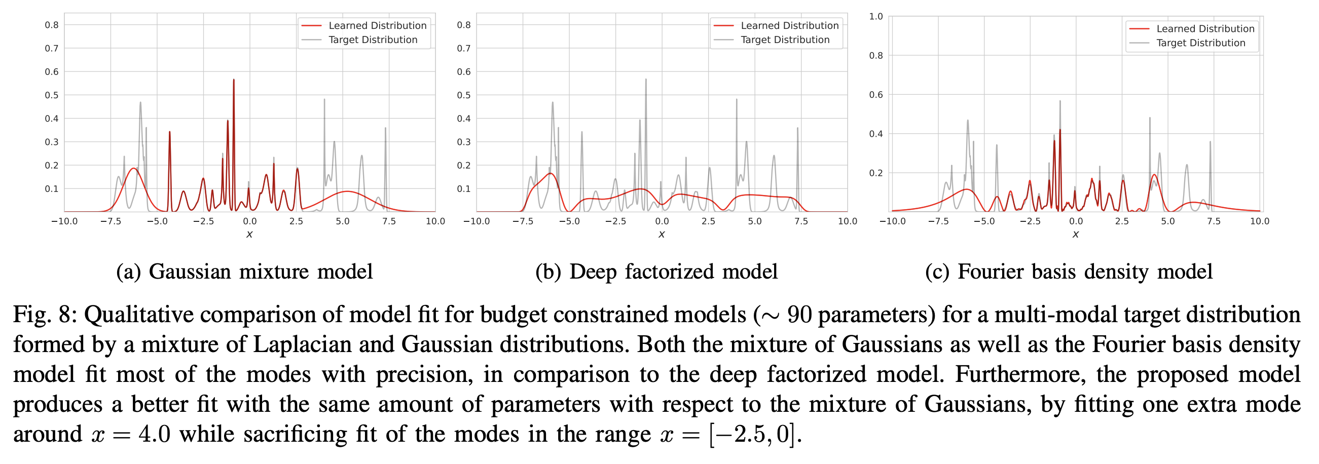] Comparison of GMM, DFP, and FBDM performance

The author's guess as to why FBDM has this advantage is that its imaginary-exponential form is, in essence, trigonometric, and unlike the negative exponentials in GMM, it doesn't suffer from severe vanishing gradients — so gradient-based optimizers have a much better chance of finding a superior solution. Viewed this way, FBDM can also be understood as a "softmax" for continuous probability densities: both construct a probability distribution using $\exp$ as a basis, the only difference being that one uses a real exponent and the other an imaginary exponent.

Compared to GMM, FBDM naturally also has some drawbacks, such as being less intuitive, harder to sample from, and harder to generalize to higher dimensions (though DFP shares these drawbacks too). GMM is quite intuitive — it's a weighted average of finitely many normal distributions, and sampling from the probability density can be achieved through hierarchical sampling: first sample a category, then sample from the corresponding normal distribution. By contrast, FBDM has no such intuitive scheme; it seems that sampling can only be done via the inverse cumulative distribution function — that is, first computing the cumulative distribution function

\begin{equation} \Phi(x) = P(\leq x) = \int_{-1}^x p_{\theta}(x)dx = \frac{x^2-1}{2} + \frac{1}{2}\sum_{n=1}^{N} \frac{c_n}{c_0} \frac{e^{i\pi n x} - (-1)^n}{i\pi n}\end{equation}

and then $y=\Phi^{-1}(\varepsilon),\varepsilon\sim U[0,1]$ can be used to perform the sampling. As for generalizing to higher dimensions, since the normal distribution already has a natural multi-dimensional form, generalizing GMM to arbitrary dimensions is easy. But if FBDM were extended directly to $D$ dimensions, it would require $(N+1)^D$ parameters, which is clearly too complex — or, similar to decoder-only LLMs, one could convert it into multiple one-dimensional conditional probability density estimations via autoregression. In short, there are ways to do it, but they involve a lot more convoluted machinery.

Summary

This article introduced a new idea for modeling one-dimensional probability density functions using Fourier series. The key point is that, through an ingenious construction of coefficients, we constrain a Fourier series — whose range would otherwise be the complex domain — to become a non-negative function. The whole process is quite delightful and well worth studying.