Using the Dirac Function to Construct Smooth Approximations of Non-Smooth Functions

用狄拉克函数来构造非光滑函数的光滑近似 苏剑林 · 2021-10-10 · Mathematics function approximation analysis smoothness

In machine learning, we often run into non-smooth functions, but our optimization methods are typically gradient-based, which means a smooth model is usually more favorable for optimization (since the gradient is continuous). This creates a need to find smooth approximations of non-smooth functions. In fact, this blog has already touched on related topics multiple times, such as in Seeking a Smooth Maximum Function and Musings on Function Smoothing: Differentiable Approximations of Non-Differentiable Functions, but the methods discussed there weren't particularly general-purpose.

Recently, however, I learned a fairly general approach from a paper, SAU: Smooth activation function using convolution with approximate identities: using the Dirac function to construct smooth approximations. How general is it? In theory, any function with a countable number of discontinuities can have a smooth approximation constructed this way! I find this quite interesting. more

The Dirac Function

Long ago, in the post The Weird Dirac Function, we already introduced the Dirac function. In modern mathematics, the Dirac function is defined as a "functional" rather than a "function," but for most readers it's easier to just think of it as a function.

Briefly, the Dirac function $\delta(x)$ satisfies:

1. $\forall x\neq 0, \delta(x) = 0$;
2. $\delta(0) = \infty$;
3. $\int_{-\infty}^{\infty} \delta(x) dx = 1$.

Intuitively, $\delta(x)$ can be thought of as a continuous probability density function over the entire real line $\mathbb{R}$, except that the probability is nonzero only at $x=0$ — that is, both the mean and the variance are 0. So sampling from it must always yield 0, which gives us the following identity:

\begin{equation}\int_{-\infty}^{\infty} f(x)\delta(x) dx = f(0)\end{equation}

or

\begin{equation}\int_{-\infty}^{\infty} f(y)\delta(x-y) dy = f(x)\label{eq:base}\end{equation}

This is arguably the most important property of the Dirac function, and it's the identity we'll mainly rely on below.

Smooth Approximation

If we can find a smooth approximation $\varphi(x)\approx \delta(x)$ of $\delta(x)$, then according to $\eqref{eq:base}$ we have

\begin{equation}g(x) = \int_{-\infty}^{\infty} f(y)\varphi(x-y) dy \approx f(x)\end{equation}

Since $\varphi(x)$ is smooth, $g(x)$ is also smooth. In other words, $g(x)$ is a smooth approximation of $f(x)$! This is the core idea behind using a smooth approximation of the Dirac function to build a smooth approximation of $f(x)$. In this process, there aren't many restrictions on the form or continuity of $f(x)$ — for instance, $f(x)$ is allowed to have a countable number of discontinuities (such as the floor function $[x]$).

So what smooth approximations of the Dirac function are available? There are quite a few ready-made ones, for example:

\begin{equation}\delta(x) = \lim_{\sigma\to 0} \frac{e^{-x^2/2\sigma^2}}{\sqrt{2\pi}\sigma}\label{eq:g}\end{equation}

or

\begin{equation}\delta(x)=\frac{1}{\pi} \lim_{a \to 0}\frac{a}{x^2+a^2}\end{equation}

Roughly speaking, the idea is to find a non-negative bell-shaped function, like a normal distribution, and find a way to let the width of the bell shrink toward zero while keeping the integral equal to 1. Another approach is to note that

\begin{equation}\int_{-\infty}^x \delta(t)dt = \theta(x) = \left\{\begin{aligned}1,\,\, (x > 0) \\ 0,\,\, (x < 0)\end{aligned}\right.\end{equation}

That is, the integral of the Dirac function is the "unit step function" $\theta(x)$. If we can find a smooth approximation of $\theta(x)$, then differentiating it gives us a smooth approximation of the Dirac function. And a smooth approximation of $\theta(x)$ is exactly what's known as an "S-shaped" curve — for example, the sigmoid function $\sigma(x)=1/(1+e^{-x})$. So we have

\begin{equation}\delta(x) = \lim_{t\to \infty} \frac{d}{dx}\sigma(tx) = \lim_{t\to \infty} \frac{e^{tx}t}{(1+e^{tx})^2}\label{eq:s}\end{equation}

The two commonly used approximations are Equations $\eqref{eq:g}$ and $\eqref{eq:s}$.

The ReLU Activation

Now let's use the above approach as a tool to derive various smooth approximations of the ReLU activation function $\max(x,0)$.

For instance, using Equation $\eqref{eq:s}$, we get

\begin{equation}\begin{aligned} \max(x,0)\approx&\, \int_{-\infty}^{\infty} \frac{e^{t(x-y)}t}{(1+e^{t(x-y)})^2} \max(y,0) dy\\ =&\,\int_0^{\infty} \frac{e^{t(x-y)}ty}{(1+e^{t(x-y)})^2}dy=\frac{\log(1+e^{tx})}{t} \end{aligned}\end{equation}

When $t=1$, this is exactly the SoftPlus activation function.

If instead we use Equation $\eqref{eq:g}$, the result is

\begin{equation}\begin{aligned} \max(x,0)\approx&\, \int_{-\infty}^{\infty} \frac{e^{-(x-y)^2/2\sigma^2}}{\sqrt{2\pi}\sigma} \max(y,0) dy\\ =&\,\int_0^{\infty} \frac{e^{-(x-y)^2/2\sigma^2} y}{\sqrt{2\pi}\sigma}dy\\ =&\,\frac{1}{2} \left[x \,\text{erf}\left(\frac{x}{\sqrt{2} \sigma}\right)+x+\sqrt{\frac{2}{\pi }} \sigma e^{-\frac{x^2}{2 \sigma^2}}\right] \end{aligned}\end{equation}

This particular smooth approximation of ReLU doesn't appear to have been studied before.

Of course, if we're only after a smooth approximation of the ReLU function, there's an even simpler approach: note that $\max(x,0)=x\theta(x)$, where $\theta(x)$ is the unit step function mentioned earlier. So the problem reduces to finding a smooth approximation of $\theta(x)$, and we already know sigmoid is one such approximation, which quickly gives us

\begin{equation}\max(x,0)\approx x\sigma(tx)\end{equation}

When $t=1$, this is exactly the Swish activation function. And if we compute using $\eqref{eq:g}$, we get

\begin{equation}\begin{aligned} \max(x,0)\approx&\, x\int_{-\infty}^{\infty} \frac{e^{-(x-y)^2/2\sigma^2}}{\sqrt{2\pi}\sigma} \theta(y) dy\\ =&\,x\int_0^{\infty} \frac{e^{-(x-y)^2/2\sigma^2}}{\sqrt{2\pi}\sigma}dy =\frac{1}{2}\left[x + x\,\text{erf}\left(\frac{x}{\sqrt{2}\sigma}\right)\right] \end{aligned}\end{equation}

When $\sigma=1$, this is exactly the GeLU activation function.

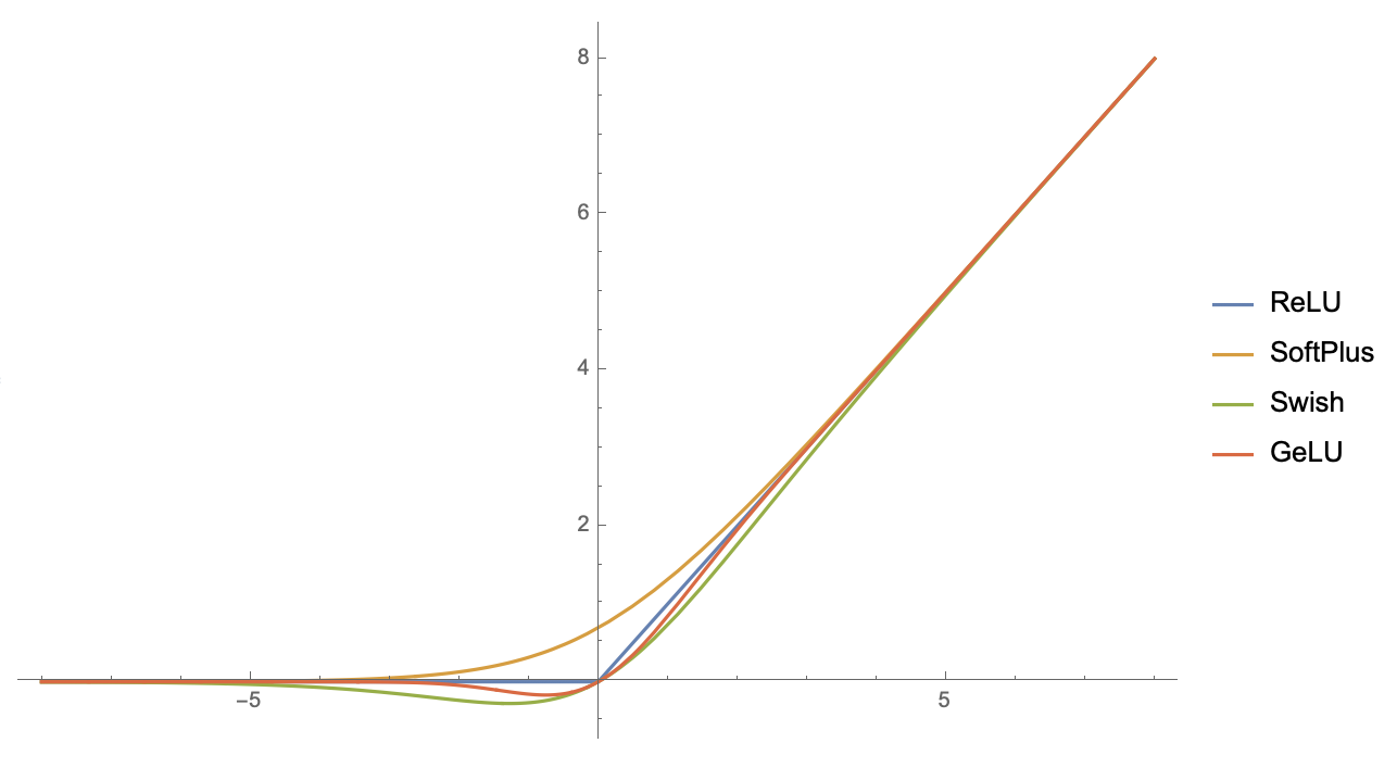Plot of the ReLU function and several of its smooth approximations

The Floor Function

Readers might feel this isn't quite satisfying yet, since everything derived above is already a known result, and can be derived without resorting to the Dirac function at all. So let's add a less trivial example: a smooth approximation of the floor function.

There are both "round up" (ceiling) and "round down" (floor) versions of the rounding function; they differ in definition but aren't fundamentally different. Here we take the floor function as our example, denoted

\begin{equation}[x] = n, \,\,\text{if and only if exists}n\in\mathbb{Z}\text{such that}x\in[n, n + 1)\end{equation}

Suppose $\varphi(x)$ is some smooth approximation of the Dirac function. Then

\begin{equation} [x]\approx \int_{-\infty}^{\infty} \varphi(x-y)[y]dy = \sum_{n=-\infty}^{\infty}n\int_n^{n+1} \varphi(x-y)dy\end{equation}

Let the antiderivative of $\varphi(x)$ be $\Phi(x)$. Then the antiderivative of $\varphi(x-y)$ with respect to $y$ is $-\Phi(x-y)$, so we have

\begin{equation}\begin{aligned}[] [x]\approx&\,\sum_{n=-\infty}^{\infty}n\big[\Phi(x-n) - \Phi(x-n-1)\big]\\ =&\,\lim_{M,N\to\infty}\sum_{n=-M}^{N}(n-1)\Phi(x-n) - n\Phi(x-n-1) + \Phi(x-n)\\ =&\,\lim_{M,N\to\infty} -N\Phi(x-N-1) - (M+1)\Phi(x+M) + \sum_{n=-M}^{N} \Phi(x-n) \end{aligned}\end{equation}

For $\Phi(x)$ we have $\Phi(-\infty)=0$ and $\Phi(\infty)=1$, so if we assume the range of interest satisfies $-M\ll x \ll N$, then $\Phi(x-N-1)\approx 0$ and $\Phi(x+N)\approx 1$, and thus in this case:

\begin{equation}\begin{aligned}[] [x]\approx&\, -M-1 + \sum_{n=-M}^{N} \Phi(x-n)\\ =&\,\sum_{n=-M}^0 \big[\Phi(x-n)-1\big] + \sum_{n=1}^N \Phi(x-n) \end{aligned}\end{equation}

Using $\Phi(x)=\sigma(tx)$ as an example, and taking $t=10,M=5,N=10$, we get the following result:

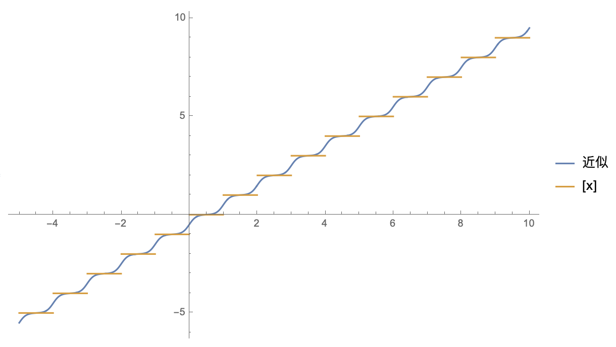The smoothing effect of the smooth approximation of the floor function

As we can see, this indeed approximates $[x]$ quite well, and increasing $t$ further improves the approximation.

Summary

This post introduced a method for constructing smooth approximations using the Dirac function, notable for its generality and lack of strict requirements on the original function. As examples, we used it to derive several common approximations of the ReLU function, as well as a smooth approximation of the floor function.