EMO: A Classification Loss Function Designed Around Optimal Transport
As is well known, the standard loss for classification tasks is cross-entropy (equivalent to maximum likelihood, MLE). It is simple and efficient, but in certain scenarios it also exposes issues such as misalignment with the evaluation metric and overconfidence. There has been a good deal of work aimed at improving on it, some of which we have covered before, such as Revisiting the Class-Imbalance Problem: The Connection Between Reweighting and Loss Hacking, How to Train Your Accuracy?, and A Simple Recipe for Alleviating Cross-Entropy Overconfidence. Since LLM training can also be understood as a per-token classification task whose default loss is likewise cross-entropy, this line of improvement work remains valuable in the current era of LLMs.
In this post, we look at a paper called EMO: Earth Mover Distance Optimization for Auto-Regressive Language Modeling, which draws on the idea of optimal transport to propose a new loss function, EMO, claimed to substantially improve LLM fine-tuning results. Let's dig into the details. more
Probability Divergence
Suppose $p_i$ is the probability the model assigns to the $i$-th class, $i=1,2,\cdots,n$, and $t$ is the target class. Then the cross-entropy loss is
\begin{equation}\mathcal{L} = - \log p_t\end{equation}
If we write the label $t$ as a one-hot distribution $\tau$ (i.e., $\tau_t=1,\tau_i=0|i\neq t, i\in[1,n]$), then this can be rewritten as
\begin{equation}\mathcal{L} = - \sum_i \tau_i\log p_i\end{equation}
This form also applies to non-one-hot labels $\tau$ (i.e., soft labels), and it is equivalent to optimizing the KL divergence of $\tau,p$:
\begin{equation}KL(\tau\Vert p) = \sum_i \tau_i\log \frac{\tau_i}{p_i} = \color{skyblue}{\sum_i \tau_i\log \tau_i} - \sum_i \tau_i\log p_i\end{equation}
Once $\tau$ is fixed, the first term on the far right is just a constant, so this is equivalent to the cross-entropy objective.
This result shows that when we perform MLE, or use cross-entropy as the loss, we are in fact minimizing the KL divergence between the target distribution and the predicted distribution. Since the KL divergence is a special case of the more general family of f-divergences (see A Brief Introduction to f-GAN: The GAN Production Workshop), it's natural to wonder whether swapping in some other f-divergence might help. Indeed, quite a few works follow exactly this line of thinking — for instance the method introduced in A Simple Recipe for Alleviating Cross-Entropy Overconfidence, whose starting point is the "Total Variation distance," itself another kind of f-divergence.
Optimal Transport
That said, every f-divergence has its own shortcomings, more or less. If we're looking for an ideal measure between probability distributions, the "Earth Mover's Distance" (EMD), grounded in optimal transport theory, is arguably the gold standard. Readers unfamiliar with it may want to check out my earlier post From the Wasserstein Distance and Duality Theory to WGAN.
In short, the Earth Mover's Distance is defined as the minimal transport cost between two distributions:
\begin{equation}\mathcal{C}[p,\tau]=\inf_{\gamma\in \Pi[p,\tau]} \sum_{i,j} \gamma_{i,j} c_{i,j} \end{equation}
Here $\gamma\in \Pi[p,\tau]$ means that $\gamma$ ranges over all joint distributions whose marginals are $p,\tau$, $c_{i,j}$ is a pre-specified cost function representing "the cost of moving mass from $i$ to $j$," and $\inf$ denotes an infimum — that is, we take the lowest possible transport cost as the measure of discrepancy between $p,\tau$. Just as replacing the f-divergence-based Vanilla GAN with the optimal-transport-based Wasserstein GAN yields better convergence properties, we might hope that replacing the classification loss with the W-distance between two distributions would likewise converge to better results.
When $\tau$ is a one-hot distribution, the target distribution collapses to a single point $t$, so there's no longer any question of optimality — there is only one possible transport plan, namely moving all the mass of $p$ to that single point $t$. In that case we simply have
\begin{equation}\mathcal{C}[p,\tau]= \sum_i p_i c_{i,t} \label{eq:emo}\end{equation}
If $\tau$ is a general soft-label distribution, then computing $\mathcal{C}[p,\tau]$ becomes a linear programming problem, which is relatively costly to solve. However, since the distribution defined by $p_i \tau_j$ also belongs to $\Pi[p,\tau]$, we have
\begin{equation}\mathcal{C}[p,\tau]=\inf_{\gamma\in \Pi[p,\tau]} \sum_{i,j} \gamma_{i,j} c_{i,j} \leq \sum_{i,j} p_i \tau_j c_{i,j} \end{equation}
This gives an easily computable upper bound, which can itself serve as the optimization objective. Equation $\eqref{eq:emo}$ then corresponds to $\tau_j = \delta_{j,t}$, where $\delta$ is the "Kronecker delta function."
Cost Function
Let's now return to the scenario the original paper actually cares about — fine-tuning LLMs, including continued pretraining and fine-tuning on downstream tasks. As mentioned at the start of this post, LLM training can be viewed as a per-token classification task (where the classes are all the tokens in the vocabulary), and each label is one-hot, so equation $\eqref{eq:emo}$ applies.
What's still missing from equation $\eqref{eq:emo}$ is the cost function $c_{i,t}$. If we simply say the cost is 1 whenever $i\neq t$, i.e., $c_{i,t}=1 - \delta_{i,t}$, then
\begin{equation}\mathcal{C}[p,\tau]= \sum_i p_i c_{i,t} = \sum_i (p_i - p_i \delta_{i, t}) = 1 - p_t\end{equation}
This is essentially a smooth approximation to maximizing accuracy (see Musings on Function Smoothing: Differentiable Approximations to Non-Differentiable Functions). But intuitively, penalizing every $i\neq t$ equally seems overly simplistic. Ideally, the cost for each different $i$ should depend on similarity — the more similar, the lower the transport cost. So we can design the transport cost as
\begin{equation}c_{i,t} = 1 - \cos(\boldsymbol{e}_i,\boldsymbol{e}_t) = 1 - \left\langle\frac{\boldsymbol{e}_i}{\Vert\boldsymbol{e}_i\Vert}, \frac{\boldsymbol{e}_t}{\Vert\boldsymbol{e}_t\Vert}\right\rangle\end{equation}
Here $\boldsymbol{e}_i,\boldsymbol{e}_t$ is a pre-obtained token embedding; in the original paper, the LM head of the pretrained model is used as the token embedding. Note that, by the definition of optimal transport, the cost function must be fixed in advance, so the token embeddings used to compute similarity must be kept frozen during training.
Once we have the cost function, we can compute
\begin{equation}\mathcal{C}[p,\tau]= \sum_i p_i c_{i,t} = \sum_i \left(p_i - p_i \left\langle\frac{\boldsymbol{e}_i}{\Vert\boldsymbol{e}_i\Vert}, \frac{\boldsymbol{e}_t}{\Vert\boldsymbol{e}_t\Vert}\right\rangle\right) = 1 - \left\langle \sum_i p_i \frac{\boldsymbol{e}_i}{\Vert\boldsymbol{e}_i\Vert}, \frac{\boldsymbol{e}_t}{\Vert\boldsymbol{e}_t\Vert}\right\rangle\end{equation}
This is the final training loss of EMO (Earth Mover Distance Optimization). Since the embedding size is usually much smaller than the vocabulary size, computing $\sum\limits_i p_i \frac{\boldsymbol{e}_i}{\Vert\boldsymbol{e}_i\Vert}$ first significantly reduces the computational cost.
Experimental Results
Since my own LLM research is still at the pretraining stage and hasn't yet reached fine-tuning, I don't have my own experimental results to share for now, so let's just walk through the experiments from the original paper together. I have to say, the results are quite impressive.
First, there are continued-pretraining experiments on small models, where compared to cross-entropy (MLE), the improvement reaches as much as 10 points, and EMO achieves state-of-the-art across the board:
 Comparison of continued-pretraining experiments on small models
It's worth noting that the evaluation metric here is MAUVE (higher is better), introduced in MAUVE: Measuring the Gap Between Neural Text and Human Text using Divergence Frontiers, one of the automatic metrics most correlated with human evaluation. In addition, one of the baseline methods, TaiLr, was briefly discussed in our earlier post A Simple Recipe for Alleviating Cross-Entropy Overconfidence.
Some readers might wonder whether EMO only looks better because of a favorable choice of evaluation metric. Surprisingly, that's not the case — models trained with EMO even achieve better perplexity (PPL), which is much more closely tied to MLE:
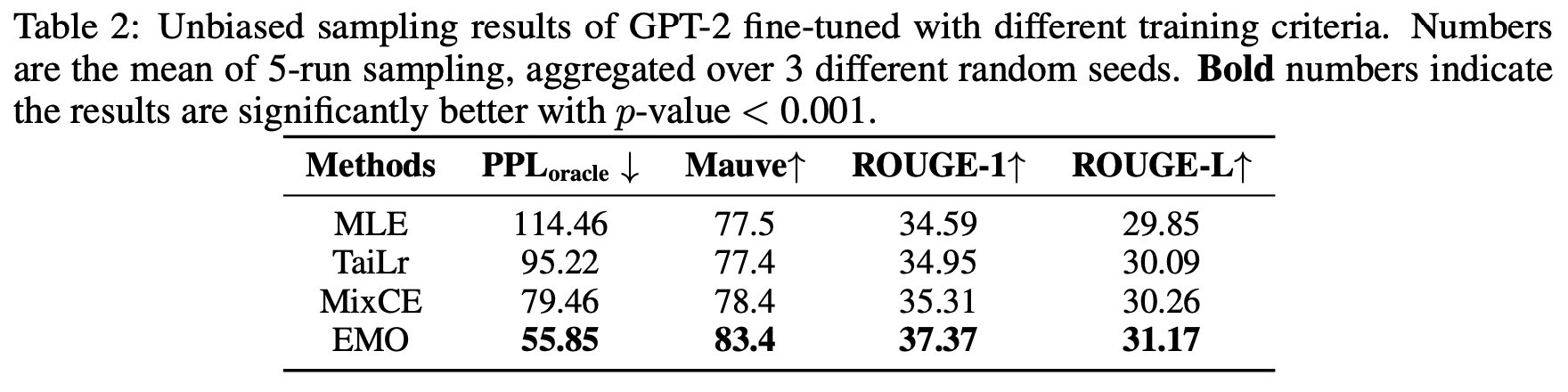 Comparison across different evaluation metrics
Next are results from fine-tuning LLaMA-7B/13B on downstream tasks for few-shot evaluation, which are likewise impressive:
 Results of fine-tuning LLaMA-7B/13B on downstream tasks
Finally, the paper compares results across different model sizes and data scales, showing that EMO performs well consistently across various model and data scales:
 Results across different model sizes/data scales
My Own Thoughts
Overall, the original paper's "report card" looks quite impressive and is well worth trying out. The one lingering concern is that the data scale used in the paper's experiments isn't actually very large, so it's unclear whether the gap between EMO and MLE would shrink as the data scale grows further.
In my view, the reason EMO achieves better results is that, by computing similarity through embeddings, it assigns more sensible losses to "near-synonym" tokens, making the model's learning process more reasonable overall. Although LLM training is formally a classification task, it isn't really a simple right-or-wrong problem — it's not the case that a sentence becomes unreasonable just because the next predicted token differs from the label token. Hence, incorporating semantic similarity into the loss design should indeed help with LLM training. One can further conjecture that the larger the vocabulary size and the coarser the token granularity, the more effective EMO should be, since a larger vocabulary means more potential "near-synonyms."
Of course, introducing semantic similarity also means EMO isn't suitable for training from scratch, since it requires a trained LM head to serve as the token embedding. One possible workaround would be to pre-train the token embeddings using some other method, such as the classic Word2Vec approach. But this carries a risk: token embeddings trained via a classical method might lower the ceiling of the LLM's ultimate capability (due to potential inconsistency with how the model itself would represent tokens).
Moreover, even if the token embeddings themselves are fine, using EMO alone from scratch might still suffer from slow convergence. This follows from the loss-function perspective I proposed at the end of How to Train Your Accuracy?:
First find a smooth approximation to the evaluation metric, ideally expressible as an expectation over samples; then gradually push the loss to infinity in the direction of errors (to ensure the model pays more attention to misclassified samples), while also ensuring a first-order approximation to the original form in the direction of correctness.
In other words, to guarantee convergence speed when training from scratch, the loss should ideally diverge to infinity in the direction of errors — and EMO clearly does not satisfy this. So when applying EMO to training from scratch, it would most likely need to be combined with MLE in some weighted fashion, in order to balance convergence speed against final performance.
Summary
This post introduced a new "alternative" to the cross-entropy loss — EMO, built on the idea of optimal transport. Unlike many past incremental improvements, EMO delivers a fairly substantial gain in LLM fine-tuning experiments.
Translated automatically with claude-sonnet-5; all equations are reproduced verbatim from the source. Copyright remains with the original author.