Revisiting Shared Output Embeddings in Language Models

语言模型输出端共享Embedding的重新探索 苏剑林 · 2023-07-20 · Machine Learning language model initialization

When pretraining first took off, reusing the Embedding weights at the output end of a language model was a very common practice—BERT, the first version of T5, and early versions of GPT all did this. This was because, when the model backbone is not large but the vocabulary is huge, the Embedding layer's parameter count is substantial; adding an independent weight matrix of the same size at the output would cause GPU memory consumption to spike. However, as model sizes have grown, the Embedding layer's share of the total parameter count has shrunk, and studies such as Rethinking embedding coupling in pre-trained language models have shown that sharing embeddings can have some negative effects. As a result, the practice of sharing embeddings has become increasingly rare.

This post aims to analyze the problems that can arise when sharing Embedding weights, and to explore how to initialize and parameterize things more effectively. Although shared embeddings may seem "outdated" by now, this remains an interesting research question to dig into. more

Sharing Weights

The practice of reusing Embedding weights at the output end of a language model is known in English as "Tied Embeddings" or "Coupled Embeddings." The idea is that the Embedding matrix and the projection matrix that maps hidden states to logits at the output are the same size (differing only by a transpose), and since this parameter matrix is fairly large, to avoid unnecessary waste, the two are simply made to share the same weights, as shown in the figure below:

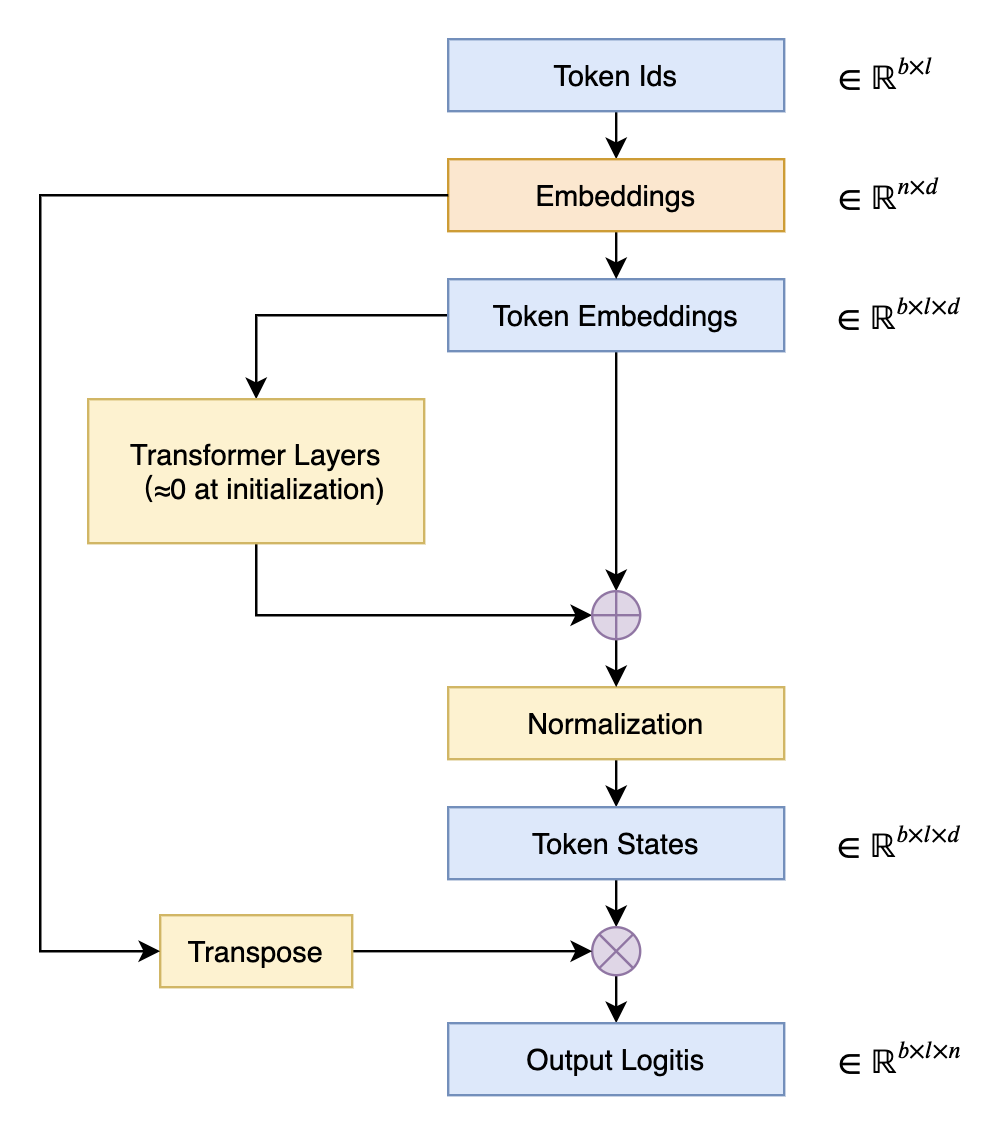Diagram of a Transformer with shared Embedding weights

The most immediate consequence of sharing embeddings may be that it causes the initial pretraining loss to be very large. This is because we typically use techniques like DeepNorm to reduce training difficulty, and these all initialize the model's residual branches to be close to zero. In other words, at the initial stage the model behaves approximately like an identity function, which makes the initial model equivalent to a 2-gram model with shared embeddings. Next, we'll work out why such a 2-gram model has such a large loss, and analyze some solutions.

Preliminaries

Before diving into the derivation proper, we need to establish some basic results.

First, we should be clear that we're mainly analyzing results at the initial stage, when the weights have all been sampled i.i.d. from some distribution with "mean 0 and variance $\sigma^2$." This lets us estimate certain summed quantities via their expectations. For example, for $\boldsymbol{w}=(w_1,w_2,\cdots,w_d)$, we have

\begin{equation}\mathbb{E}\left[\Vert \boldsymbol{w}\Vert^2\right] = \mathbb{E}\left[\sum_i w_i^2\right] = \sum_i \mathbb{E}\left[w_i^2\right] = d\sigma^2\label{eq:norm}\end{equation}

so we can take $\Vert \boldsymbol{w}\Vert\approx \sqrt{d}\sigma$. How large is the error, though? We can gauge this via its variance. To do so, let's first compute its second moment:

\begin{equation}\begin{aligned}\mathbb{E}\left[\Vert \boldsymbol{w}\Vert^4\right] =&\, \mathbb{E}\left[\left(\sum_i w_i^2\right)^2\right] = \mathbb{E}\left[\sum_i w_i^4 + \sum_{i,j|i\neq j} w_i^2 w_j^2\right] \\ =&\, \sum_i \mathbb{E}\left[w_i^4\right] + \sum_{i,j|i\neq j} \mathbb{E}\left[w_i^2\right] \mathbb{E}\left[w_j^2\right] \\ =&\, d\,\mathbb{E}\left[w^4\right] + d(d-1) \sigma^4 \\ \end{aligned}\end{equation}

If the sampling distribution is Gaussian, we can directly compute $\mathbb{E}\left[w^4\right]=3\sigma^4$, so

\begin{equation}\mathbb{V}ar\left[\Vert \boldsymbol{w}\Vert^2\right] = \mathbb{E}\left[\Vert \boldsymbol{w}\Vert^4\right] - \mathbb{E}\left[\Vert \boldsymbol{w}\Vert^2\right]^2 = 2d\sigma^4\end{equation}

The size of this variance also reflects how good the approximation $\Vert \boldsymbol{w}\Vert\approx \sqrt{d}\sigma$ is—that is, the smaller the original sampling variance $\sigma^2$, the better the approximation. In particular, a common choice for the sampling variance is $1/d$ (corresponding to $\Vert \boldsymbol{w}\Vert\approx 1$, i.e., a unit vector), and substituting this into the above expression gives $2/d$, meaning that the higher the dimension, the better the approximation. Also, if the sampling distribution isn't Gaussian, we could recompute $\mathbb{E}\left[w^4\right]$ directly for that distribution, or simply use the Gaussian result as a reference—either way it's just an estimate.

If $\boldsymbol{v}=(v_1,v_2,\cdots,v_d)$ is another i.i.d. vector, we can use the same method to estimate the inner product, giving

\begin{equation}\mathbb{E}\left[\boldsymbol{w}\cdot\boldsymbol{v}\right] = \mathbb{E}\left[\sum_i w_i v_i\right] = \sum_i \mathbb{E}\left[w_i\right] \mathbb{E}\left[v_i\right] = 0\label{eq:dot}\end{equation}

and

\begin{equation}\begin{aligned}\mathbb{E}\left[(\boldsymbol{w}\cdot\boldsymbol{v})^2\right] =&\, \mathbb{E}\left[\left(\sum_i w_i v_i\right)^2\right] = \mathbb{E}\left[\sum_i w_i^2 v_i^2 + \sum_{i,j|i\neq j} w_i v_i w_j v_j\right] \\ =&\, \sum_i \mathbb{E}\left[w_i^2\right]\mathbb{E}\left[w_j^2\right] + \sum_{i,j|i\neq j} \mathbb{E}\left[w_i\right]\mathbb{E}\left[v_i\right]\mathbb{E}\left[w_j\right]\mathbb{E}\left[v_j\right] \\ =&\, d \sigma^4 \\ \end{aligned}\end{equation}

Likewise, taking $\sigma^2=1/d$ gives a variance of $1/d^3$, and again the approximation improves with dimension. The two results above are essentially statistical versions of the conclusions in The Distribution of the Angle Between Two Random Vectors in n-Dimensional Space and The Amazing Johnson-Lindenstrauss Lemma: Theory.

Loss Analysis

For a language model, the final goal is to output, for each token, a distribution over $n$ categories, where $n$ is the vocabulary size. Suppose we simply output a uniform distribution, i.e., every token has probability $1/n$; it's easy to compute that the cross-entropy loss will then be $\log n$. This means that a reasonable initialization shouldn't produce an initial loss that significantly exceeds $\log n$, since $\log n$ represents the most naive uniform-distribution baseline—significantly exceeding $\log n$ would mean doing distinctly worse than a uniform distribution, which is like deliberately making mistakes and clearly unreasonable.

So why does sharing embeddings lead to this outcome? Suppose the initial Embedding is $\{\boldsymbol{w}_1,\boldsymbol{w}_2,\cdots,\boldsymbol{w}_n\}$. As mentioned earlier, at the initial stage the residual branch is close to zero, so given an input token $i$, the model output is just the Embedding after normalization, $\boldsymbol{w}_i$. The usual normalization is Layer Norm or RMS Norm; since the initialization distribution is zero-mean, Layer Norm and RMS Norm are roughly equivalent, so the output is

\begin{equation}\frac{\boldsymbol{w}_i}{\Vert\boldsymbol{w}_i\Vert \big/\sqrt{d}} = \frac{\boldsymbol{w}_i}{\sigma}\end{equation}

Next, reusing the Embedding, taking the inner product and applying Softmax, the resulting distribution is essentially

\begin{equation}p(j|i) = \frac{e^{\boldsymbol{w}_i\cdot \boldsymbol{w}_j / \sigma}}{\sum\limits_k e^{\boldsymbol{w}_i\cdot \boldsymbol{w}_k / \sigma}}\end{equation}

and the corresponding loss function is

\begin{equation}-\log p(j|i) = \log \sum\limits_k e^{\boldsymbol{w}_i\cdot \boldsymbol{w}_k / \sigma} - \boldsymbol{w}_i\cdot \boldsymbol{w}_j \big/ \sigma\end{equation}

Since the task of a language model is to predict the next token, and we know that the fraction of repeated-token ("reduplicated word") cases in natural sentences is small, we can basically assume $j\neq i$, so by the result $\eqref{eq:dot}$ we have $\boldsymbol{w}_i\cdot \boldsymbol{w}_j\approx 0$. Hence the initial loss function is

\begin{equation}-\log p(j|i) \approx \log \sum_k e^{\boldsymbol{w}_i\cdot \boldsymbol{w}_k / \sigma}=\log \left(e^{\boldsymbol{w}_i\cdot \boldsymbol{w}_i / \sigma} + \sum\limits_{k|k\neq i} e^{\boldsymbol{w}_i\cdot \boldsymbol{w}_k / \sigma}\right)\approx\log \left(e^{d \sigma} + (n-1)\right)\label{eq:loss}\end{equation}

The $\approx$ term above again makes use of Equations $\eqref{eq:norm}$ and $\eqref{eq:dot}$. The commonly used initialization variance $\sigma^2$ is either a constant or scales as $1/d$ (in which case $e^{d \sigma}=e^{\sqrt{d}}$); either way, when $d$ is large, $e^{d \sigma}$ dominates, so the loss ends up on the order of $\log e^{d\sigma}=d\sigma$, which easily exceeds the uniform-distribution baseline of $\log n$.

Some Countermeasures

Based on the derivation above, we can now design some targeted countermeasures. The most direct approach is to adjust the initialization: according to Equation $\eqref{eq:loss}$, we just need $e^{d\sigma}=n$, so that the initial loss becomes of order $\log n$—that is, we need to change the initialization standard deviation to $\sigma=(\log n)/d$.

Generally speaking, we'd like the initialization variance of the parameters to be as large as possible, since this makes gradient underflow less likely; and $\sigma=(\log n)/d$ can sometimes end up being too small. So let's take a different approach: it's clear that the reason Equation $\eqref{eq:loss}$ ends up being too large is that the term $e^{\boldsymbol{w}_i\cdot \boldsymbol{w}_i / \sigma}$ appears—since the two $\boldsymbol{w}_i$'s are identical, their inner product becomes a squared norm and thus grows large. If we could make them different, this dominant term would disappear.

The simplest way to do this, of course, is to simply not share the Embedding—in which case we'd have $e^{\boldsymbol{w}_i\cdot \boldsymbol{v}_i / \sigma}$ instead of $e^{\boldsymbol{w}_i\cdot \boldsymbol{w}_i / \sigma}$, using $\eqref{eq:dot}$ instead of $\eqref{eq:norm}$ as the approximation, so Equation $\eqref{eq:loss}$ asymptotically approaches $\log n$. If we still want to keep the Embedding shared, we can add an orthogonally-initialized projection layer right after the final normalization, so that $e^{\boldsymbol{w}_i\cdot \boldsymbol{w}_i / \sigma}$ becomes $e^{(\boldsymbol{w}_i\boldsymbol{P})\cdot \boldsymbol{w}_i / \sigma}$. By the Johnson-Lindenstrauss lemma, a randomly projected vector behaves approximately like an independent vector, so this again approximates the non-shared case—this is in fact how BERT handles it. In particular, this projection layer can also, more generally, include a bias term and an activation function.

If we don't want to introduce even a small amount of extra parameters, we can instead consider "shuffling" the various dimensions of $\boldsymbol{w}_i$ after normalization, for example

\begin{equation}\mathcal{S}[\boldsymbol{w}] = \boldsymbol{w}[d/2:]\circ\boldsymbol{w}[:d/2]\end{equation}

where $\circ$ denotes concatenation; then $\mathcal{S}[\boldsymbol{w}_i]$ and $\boldsymbol{w}_i$ are also close to orthogonal, so their inner product is again approximately 0. This is equivalent (at the initial stage) to splitting the original $n\times d$ Embedding matrix into two $n\times (d/2)$ matrices and building a non-shared-Embedding 2-gram model out of them. We could also consider other shuffling operations—for instance, the reshape-then-transpose-then-reshape-back trick used in ShuffleNet.

In my own experiments, simply changing the initialization standard deviation to $\sigma=(\log n)/d$ converged the slowest; the other methods converged at roughly similar rates, and in terms of final performance, all methods seemed to end up more or less the same.

Summary

This post revisited the practice of sharing Embedding weights at the output end of language models, worked out why directly reusing the Embedding for output projection can lead to an excessively large loss, and discussed several ways to address this.