Multi-Task Learning Ramblings (II): The Business of Gradients
In Multi-Task Learning Ramblings (I): In the Name of Loss, we took an initial look at multi-task learning from the perspective of the loss function, and eventually found that if we want the result to have both scale invariance and translation invariance, using the reciprocal of the gradient norm as the task weight is a fairly simple choice. We then analyzed that this design is equivalent to normalizing each task's gradient individually before summing them, which means the "battlefield" of multi-task learning has shifted from the loss function to the gradient: it looks like we're designing loss functions, but we're actually designing better gradients — so to speak, "in the name of loss, but in the business of gradients."
So what standard should a "better gradient" satisfy? How do we go about designing one? In this post, we'll look at multi-task learning from the gradient perspective, and try to construct multi-task learning algorithms directly from the idea of designing gradients.
Overall Approach
As we know, for single-task learning, the standard optimization method is gradient descent — but how is it actually derived? Can the same reasoning be applied directly to multi-task learning? That's the question this section aims to answer. more
Direction of Descent
Actually, we already answered the first question in A More Holistic View of Optimization Algorithms from a Dynamical Systems Perspective (III). Suppose the loss function is $\mathcal{L}$, the current parameters are $\boldsymbol{\theta}$, and we want to design a parameter increment $\Delta\boldsymbol{\theta}$ such that the loss function becomes smaller, i.e. $\mathcal{L}(\boldsymbol{\theta}+\Delta\boldsymbol{\theta}) < \mathcal{L}(\boldsymbol{\theta})$. To this end, we consider a first-order expansion:
\begin{equation}\mathcal{L}(\boldsymbol{\theta}+\Delta\boldsymbol{\theta})\approx \mathcal{L}(\boldsymbol{\theta}) + \langle \nabla_{\boldsymbol{\theta}}\mathcal{L}, \Delta\boldsymbol{\theta}\rangle \label{eq:approx-1}\end{equation}
Assuming this approximation is accurate enough, $\mathcal{L}(\boldsymbol{\theta}+\Delta\boldsymbol{\theta}) < \mathcal{L}(\boldsymbol{\theta})$ implies $\langle \nabla_{\boldsymbol{\theta}}\mathcal{L}, \Delta\boldsymbol{\theta}\rangle < 0$, i.e. the update must make an angle of at least 90 degrees with the gradient. Among all such choices, the most natural one is
\begin{equation}\Delta\boldsymbol{\theta} = -\eta \nabla_{\boldsymbol{\theta}}\mathcal{L}\end{equation}
This is exactly gradient descent: the update takes the opposite direction of the gradient, where $\eta > 0$ is the learning rate.
No Exceptions
Back to multi-task learning: if we assume every task is equally important, we can interpret this assumption as requiring that at every update step, $\mathcal{L}_1,\mathcal{L}_2,\cdots,\mathcal{L}_n$ all decrease or stay the same. If, once the parameters reach $\boldsymbol{\theta}^*$, any further change would cause some $\mathcal{L}_i$ to increase, then we say $\boldsymbol{\theta}^*$ is a Pareto-optimal solution. In plain terms, Pareto optimality means we cannot sacrifice one task to improve another — the tasks are not "competing" against each other.
Assuming the approximation $\eqref{eq:approx-1}$ still holds, finding a Pareto-optimal point means we need to find $\Delta\boldsymbol{\theta}$ satisfying
\begin{equation}\left\{\begin{aligned} &\langle \nabla_{\boldsymbol{\theta}}\mathcal{L}_1, \Delta\boldsymbol{\theta}\rangle \leq 0\\ &\langle \nabla_{\boldsymbol{\theta}}\mathcal{L}_2, \Delta\boldsymbol{\theta}\rangle \leq 0\\ &\quad \vdots \\ &\langle \nabla_{\boldsymbol{\theta}}\mathcal{L}_n, \Delta\boldsymbol{\theta}\rangle \leq 0\\ \end{aligned}\right.\end{equation}
Notice this system always has the trivial solution $\Delta\boldsymbol{\theta}=\boldsymbol{0}$, so the feasible region of the above inequalities is never empty. What we really care about is whether there exists a nonzero solution within this feasible region: if there is, we take it as the update direction; if not, we may already have reached a Pareto-optimal point (this is a necessary but not sufficient condition), and we call this state a Pareto-stationary point.
Solution Algorithms
For convenience, let's denote $\boldsymbol{g}_i=\nabla_{\boldsymbol{\theta}}\mathcal{L}_i$. We seek a vector $\boldsymbol{u}$ such that for all $i$, $\langle \boldsymbol{g}_i, \boldsymbol{u}\rangle \geq 0$ holds, and then, just like in single-task gradient descent, we can take $\Delta\boldsymbol{\theta}=-\eta\boldsymbol{u}$ as the update. If there are only two tasks, one can verify that $\boldsymbol{u}=\boldsymbol{g}_1/\Vert\boldsymbol{g}_1\Vert + \boldsymbol{g}_2/\Vert\boldsymbol{g}_2\Vert$ automatically satisfies $\langle \boldsymbol{g}_1, \boldsymbol{u}\rangle \geq 0$ and $\langle \boldsymbol{g}_2, \boldsymbol{u}\rangle \geq 0$ — in other words, for two-task learning, the gradient normalization discussed earlier already achieves a Pareto-stationary point.
When the number of tasks exceeds two, things get a bit more complicated. Here we introduce two solution methods: the first is a derivation the author worked out independently, and the second is the "official answer" given by Multi-Task Learning as Multi-Objective Optimization.
Reformulating the Problem
First, let's reformulate the problem further. Note that
\begin{equation}\forall i, \langle \boldsymbol{g}_i, \boldsymbol{u}\rangle \geq 0\quad\Leftrightarrow\quad \min_i \langle \boldsymbol{g}_i, \boldsymbol{u}\rangle \geq 0\label{eq:q-0}\end{equation}
So we only need to maximize the smallest of these $\langle \boldsymbol{g}_i, \boldsymbol{u}\rangle$ values in order to find the ideal $\boldsymbol{u}$, i.e. the problem becomes
\begin{equation}\max_{\boldsymbol{u}}\min_i \langle \boldsymbol{g}_i, \boldsymbol{u}\rangle \end{equation}
But this is a bit dangerous, because if there really does exist a nonzero $\boldsymbol{u}$ such that $\min\limits_i \langle \boldsymbol{g}_i, \boldsymbol{u}\rangle > 0$, then letting the norm of $\boldsymbol{u}$ tend to positive infinity would send the maximum value to infinity as well. So for stability, we need to add a regularization term, and consider instead
\begin{equation}\max_{\boldsymbol{u}}\min_i \langle \boldsymbol{g}_i, \boldsymbol{u}\rangle - \frac{1}{2}\Vert \boldsymbol{u}\Vert^2\label{eq:q-1}\end{equation}
This way, an infinite-norm $\boldsymbol{u}$ can no longer be an optimal solution. Note that substituting $\boldsymbol{u}=0$ gives $\min\limits_i \langle \boldsymbol{g}_i, \boldsymbol{u}\rangle - \frac{1}{2}\Vert \boldsymbol{u}\Vert^2=0$, so if we let the optimal solution of $\boldsymbol{u}$ maximizing $\max$ be $\boldsymbol{u}^*$, then it must satisfy
\begin{equation}\min_i \langle \boldsymbol{g}_i, \boldsymbol{u}^*\rangle - \frac{1}{2}\Vert \boldsymbol{u}^*\Vert^2\geq 0\quad\Leftrightarrow\quad \min_i \langle \boldsymbol{g}_i, \boldsymbol{u}^*\rangle \geq \frac{1}{2}\Vert \boldsymbol{u}^*\Vert^2\geq 0\end{equation}
Therefore the solution to problem $\eqref{eq:q-1}$ must be a solution satisfying condition $\eqref{eq:q-0}$, and if it is a nonzero solution, its negative direction is necessarily a direction that makes every task's loss decrease.
Smooth Approximation
Now let's introduce the first approach to solving problem $\eqref{eq:q-1}$. It assumes the reader, like the author, is not particularly familiar with solving min-max problems, so we replace the $\min$ in the first step with a smooth approximation (see In Search of a Smooth Maximum Function), i.e.
\begin{equation}\min_i \langle \boldsymbol{g}_i, \boldsymbol{u}\rangle \approx -\frac{1}{\lambda}\log\sum_i e^{-\lambda \langle \boldsymbol{g}_i, \boldsymbol{u}\rangle}\,\,\big(\text{for sufficiently large}\lambda\big)\end{equation}
We can then first solve
\begin{equation}\max_{\boldsymbol{u}}-\frac{1}{\lambda}\log\sum_i e^{-\lambda \langle \boldsymbol{g}_i, \boldsymbol{u}\rangle} - \frac{1}{2}\Vert \boldsymbol{u}\Vert^2\end{equation}
and then take the limit $\lambda\to\infty$. This converts the problem into an unconstrained maximization problem for a single function — we can just take the gradient and set it to zero, giving
\begin{equation}\frac{\sum\limits_i e^{-\lambda \langle \boldsymbol{g}_i, \boldsymbol{u}\rangle} \boldsymbol{g}_i}{\sum\limits_i e^{-\lambda \langle \boldsymbol{g}_i, \boldsymbol{u}\rangle}} = \boldsymbol{u}\end{equation}
Assuming the various $\langle \boldsymbol{g}_i, \boldsymbol{u}\rangle$ differ by more than an order of magnitude of $\mathcal{O}(1/\lambda)$, then when $\lambda\to\infty$, the above expression is effectively
\begin{equation}\boldsymbol{u} = \boldsymbol{g}_{\tau},\quad \tau = \mathop{\text{argmin}}_i \langle \boldsymbol{g}_i, \boldsymbol{u}\rangle\end{equation}
However, if we iterate directly according to $\boldsymbol{u}^{(k+1)} = \boldsymbol{g}_{\tau},\tau = \mathop{\text{argmin}}\limits_i \langle \boldsymbol{g}_i, \boldsymbol{u}^{(k)}\rangle$, it's very likely to oscillate, because this rule asks us to find the $\boldsymbol{g}_i$ that minimizes $\langle \boldsymbol{g}_i, \boldsymbol{u}^{(k)}\rangle$ and use it as $\boldsymbol{u}^{(k+1)}$ — say this turns out to be $\boldsymbol{u}^{(k+1)}=\boldsymbol{g}_{i^*}$. Then at the next step, the $\boldsymbol{g}_i$ that minimizes $\langle \boldsymbol{g}_i, \boldsymbol{u}^{(k+1)}\rangle=\langle \boldsymbol{g}_i, \boldsymbol{g}_{i^*}\rangle$ is quite likely to no longer be $\boldsymbol{g}_{i^*}$; instead, $\boldsymbol{g}_{i^*}$ might now be the largest one.
Intuitively, although the above algorithm oscillates, it should still be oscillating around the optimal point $\boldsymbol{u}^*$, so if we average all the results produced during this oscillation, we should recover the optimal point. This suggests that the iteration scheme converging to the optimum is
\begin{equation}\boldsymbol{u}^{(k+1)} = \frac{k \boldsymbol{u}^{(k)} + \boldsymbol{g}_{\tau}}{k + 1},\quad \tau = \mathop{\text{argmin}}_i \langle \boldsymbol{g}_i, \boldsymbol{u}^{(k)}\rangle\label{eq:sol-1}\end{equation}
Notice that at each step we're adding some $\boldsymbol{g}_i$, so the final $\boldsymbol{u}^*$ must be a weighted average of the various $\boldsymbol{g}_i$, i.e. there exist $\alpha_1,\alpha_2,\cdots,\alpha_n\geq 0$ with $\alpha_1 + \alpha_2 + \cdots + \alpha_n =1$, such that
\begin{equation}\boldsymbol{u}^* = \sum_i \alpha_i \boldsymbol{g}_i\end{equation}
We can also interpret $\alpha_1,\alpha_2,\cdots,\alpha_n$ as the current optimal weight assignment across the various $\mathcal{L}_i$.
The Dual Problem
The advantage of the smooth-approximation trick is that it is simple and intuitive, requiring no deep background in optimization theory. Still, it is ultimately a "non-mainstream" approach, with quite a few points that aren't fully rigorous (though the result is correct). Let's now look at the "official answer," based on duality.
First, define $\mathbb{P}^n$ as the set of all discrete distributions over $n$ elements, i.e.
\begin{equation}\mathbb{P}^n = \left\{(\alpha_1,\alpha_2,\cdots,\alpha_n)\left|\alpha_1,\alpha_2,\cdots,\alpha_n\geq 0, \sum_i \alpha_i = 1\right.\right\}\end{equation}
It's then easy to verify that
\begin{equation}\min_i \langle \boldsymbol{g}_i, \boldsymbol{u}\rangle = \min_{\alpha\in\mathbb{P}^n}\left\langle \tilde{\boldsymbol{g}}(\alpha), \boldsymbol{u}\right\rangle,\quad \tilde{\boldsymbol{g}}(\alpha) = \sum_i \alpha_i \boldsymbol{g}_i\end{equation}
Therefore problem $\eqref{eq:q-1}$ is equivalent to
\begin{equation}\max_{\boldsymbol{u}}\min_{\alpha\in\mathbb{P}^n}\left\langle \tilde{\boldsymbol{g}}(\alpha), \boldsymbol{u}\right\rangle - \frac{1}{2}\Vert \boldsymbol{u}\Vert^2\label{eq:q-2}\end{equation}
The function above is concave in $\boldsymbol{u}$ and convex in $\alpha$, and the feasible regions for both $\boldsymbol{u},\alpha$ are convex sets (the weighted average of any two points in the set remains in the set). So by von Neumann's minimax theorem, the $\min$ and $\max$ in equation $\eqref{eq:q-2}$ can be swapped, i.e. it is equivalent to
\begin{equation}\min_{\alpha\in\mathbb{P}^n}\max_{\boldsymbol{u}}\left\langle \tilde{\boldsymbol{g}}(\alpha), \boldsymbol{u}\right\rangle - \frac{1}{2}\Vert \boldsymbol{u}\Vert^2 = \min_{\alpha\in\mathbb{P}^n}\frac{1}{2}\left\Vert\tilde{\boldsymbol{g}}(\alpha)\right\Vert^2\label{eq:q-3}\end{equation}
The equality on the right-hand side holds because the $\max$ part is just an unconstrained quadratic maximization problem, whose solution $\boldsymbol{u}^* = \tilde{\boldsymbol{g}}(\alpha)$ can be computed directly. So what remains is just $\min$, and the problem becomes finding a weighted average of $\boldsymbol{g}_1,\boldsymbol{g}_2,\cdots,\boldsymbol{g}_n$ that has minimal norm.
When $n=2$, the solution is fairly simple — it amounts to constructing the altitude of a triangle, as shown in the figure below:
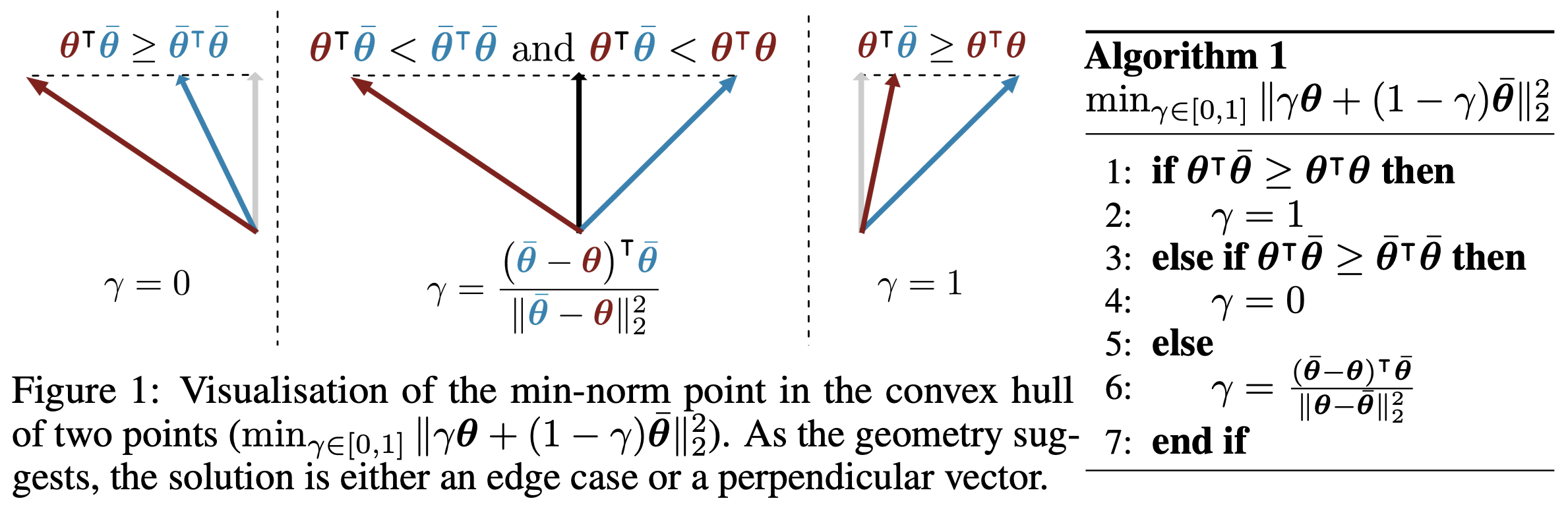 Solution algorithm and geometric meaning when n=2
When $n > 2$, we can use the Frank–Wolfe algorithm to reduce it to a series of cases with $n=2$, solved iteratively. The Frank–Wolfe algorithm can be understood as a constrained gradient descent algorithm, well suited to cases where the feasible region of the parameters is a convex set — a full explanation would take too much space, so we won't go into detail here; interested readers can look it up. Briefly, the Frank–Wolfe algorithm first linearizes the objective to find the next update direction $e_{\tau}$, where $\tau = \mathop{\text{argmin}}\limits_i \langle \boldsymbol{g}_i, \tilde{\boldsymbol{g}}(\alpha)\rangle$ and $e_{\tau}$ is the one-hot vector with a 1 at position $\tau$, and then searches by interpolating between $\alpha$ and $e_{\tau}$, picking whichever gives the best result. So the iteration proceeds as
\begin{equation}\left\{\begin{aligned} &\tau = \mathop{\text{argmin}}_i \langle \boldsymbol{g}_i, \tilde{\boldsymbol{g}}(\alpha^{(k)})\rangle\\ &\gamma = \mathop{\text{argmin}}_{\gamma} \left\Vert\tilde{\boldsymbol{g}}((1-\gamma)\alpha^{(k)} + \gamma e_{\tau})\right\Vert^2 = \mathop{\text{argmin}}_{\gamma} \left\Vert(1-\gamma)\tilde{\boldsymbol{g}}(\alpha^{(k)}) + \gamma \boldsymbol{g}_{\tau}\right\Vert^2\\ &\alpha^{(k+1)} = (1-\gamma)\alpha^{(k)} + \gamma e_{\tau} \end{aligned}\right.\end{equation}
where solving for $\gamma$ is exactly a special case of $n=2$, which can be solved with the algorithm in the screenshot above. If $\gamma$ is not obtained via search but instead fixed at $1/(k+1)$, the result is equivalent to $\eqref{eq:sol-1}$ — this is also a simplified version of the Frank–Wolfe algorithm. In other words, the result we obtained via smooth approximation is equivalent to that of the simplified Frank–Wolfe algorithm.
Removing the Constraint
Actually, for solving problem $\eqref{eq:q-3}$, in principle we could also remove the constraint and solve it directly with gradient descent. For example, we could directly set the parameter $\beta_1,\beta_2,\cdots,\beta_n\in\mathbb{R}$ and
\begin{equation}\alpha_i = \frac{e^{\beta_i}}{Z},\quad Z = \sum_i e^{\beta_i}\end{equation}
which converts the problem into
\begin{equation}\min_{\beta} \frac{1}{2Z^2}\left\Vert \sum_i e^{\beta_i} \boldsymbol{g}_i\right\Vert^2\end{equation}
This is an unconstrained optimization problem that ordinary gradient descent can solve. Yet, for some reason, the author doesn't seem to have seen this approach used anywhere (perhaps people don't want to tune yet another learning rate?).
Some Tricks
In the previous section, we gave two schemes for finding the update direction toward a Pareto-stationary point. Both require, at every training step, running several additional iterations to determine the weight for each task before we can even update the model parameters. As one might imagine, this can be quite expensive computationally in practice, so we need some tricks to reduce the cost.
Gradient Inner Products
As we can see, no matter which scheme we use, the key step always involves $\mathop{\text{argmin}}\limits_i \langle \boldsymbol{g}_i, \tilde{\boldsymbol{g}}(\alpha)\rangle$, which requires iterating over the gradients to compute inner products. However, in a deep learning setting, the number of model parameters is often huge, so the gradient is an extremely high-dimensional vector — computing an inner product at every iteration is expensive. Here we can exploit the expansion
\begin{equation}\langle \boldsymbol{g}_i, \tilde{\boldsymbol{g}}(\alpha)\rangle = \left\langle \boldsymbol{g}_i, \sum_j \alpha_j \boldsymbol{g}_j \right\rangle = \sum_j \alpha_j \langle \boldsymbol{g}_i, \boldsymbol{g}_j \rangle\end{equation}
At each iteration, only $\alpha$ actually changes, so in fact $\langle \boldsymbol{g}_i, \boldsymbol{g}_j \rangle$ only needs to be computed once per training step and cached, avoiding repeated computation of these large inner products.
Shared Encoder
However, once the model grows large enough, computing each task's gradient separately and then iterating becomes impractical. If we assume the models for the different tasks share the same encoder, we can further approximate and simplify the algorithm.
Concretely, suppose the batch size is $b$, and the encoder output for the $j$-th sample is $\boldsymbol{h}_j$. Then by the chain rule we know:
\begin{equation}\boldsymbol{g}_i = \nabla_{\boldsymbol{\theta}}\mathcal{L}_i = \sum_j (\nabla_{\boldsymbol{h}_j}\mathcal{L}_i)(\nabla_{\boldsymbol{\theta}}\boldsymbol{h}_j) = \underbrace{\big(\nabla_{\boldsymbol{h}_1}\mathcal{L}_i , \cdots , \nabla_{\boldsymbol{h}_b}\mathcal{L}_i\big)}_{\nabla_{\boldsymbol{H}}\mathcal{L}_i}\underbrace{\begin{pmatrix}\nabla_{\boldsymbol{\theta}}\boldsymbol{h}_b \\ \vdots \\ \nabla_{\boldsymbol{\theta}}\boldsymbol{h}_b\end{pmatrix}}_{\nabla_{\boldsymbol{\theta}}\boldsymbol{H}}\end{equation}
Let $\boldsymbol{H} = (\boldsymbol{h}_1,\cdots,\boldsymbol{h}_b)$, so that $\boldsymbol{g}_i = (\nabla_{\boldsymbol{H}}\mathcal{L}_i) (\nabla_{\boldsymbol{\theta}}\boldsymbol{H})$, and using the matrix norm inequality we get
\begin{equation}\left\Vert\sum_i \alpha_i \boldsymbol{g}_i\right\Vert^2 = \left\Vert\sum_i \alpha_i (\nabla_{\boldsymbol{H}}\mathcal{L}_i) (\nabla_{\boldsymbol{\theta}}\boldsymbol{H})\right\Vert^2 \leq \left\Vert\sum_i \alpha_i \nabla_{\boldsymbol{H}}\mathcal{L}_i\right\Vert^2 \big\Vert \nabla_{\boldsymbol{\theta}}\boldsymbol{H}\big\Vert^2 \end{equation}
It's not hard to see that if we minimize $\left\Vert\sum\limits_i\alpha_i \nabla_{\boldsymbol{H}}\mathcal{L}_i\right\Vert^2$, the computational cost drops significantly, since this only requires the gradient with respect to the final output encoding vector, rather than the gradient with respect to all parameters. And the inequality above tells us that minimizing $\left\Vert\sum\limits_i\alpha_i \nabla_{\boldsymbol{H}}\mathcal{L}_i\right\Vert^2$ is really minimizing an upper bound on $\eqref{eq:q-3}$. As with many problems that are hard to optimize directly, we hope that minimizing the upper bound also yields a similar outcome.
That said, while this upper bound is more efficient, it also has its limitations. It's generally only suitable for multi-task learning where every sample has multiple types of labels; it doesn't apply when the training data for different tasks has no overlap (i.e. each task's labels come from different samples, and any given sample only has one type of label). In the latter case, the various $\nabla_{\boldsymbol{H}}\mathcal{L}_i$ are mutually orthogonal, so there's no interaction between tasks, and the bound fails to reflect any correlation between tasks — it becomes so loose as to be meaningless.
A Flawed Proof
The "official answer" mentioned earlier, as well as the result about optimizing the upper bound with a shared encoder, both come from the paper Multi-Task Learning as Multi-Objective Optimization. That paper goes on to try to prove that when $\nabla_{\boldsymbol{\theta}}\boldsymbol{H}$ is full rank, optimizing the upper bound also finds a Pareto-stationary point. Unfortunately, the proof in the original paper is flawed.
The proof appears in Appendix A of the original paper, and it relies on an incorrect claim:
If $\boldsymbol{M}$ is a symmetric positive-definite matrix, then $\boldsymbol{x}^{\top}\boldsymbol{y}\geq 0$ if and only if $\boldsymbol{x}^{\top}\boldsymbol{M}\boldsymbol{y}\geq 0$.
It's easy to find a counterexample: take $\boldsymbol{x}=\begin{pmatrix}1 \\ -2\end{pmatrix},\boldsymbol{y}=\begin{pmatrix}1 \\ 1\end{pmatrix},\boldsymbol{M}=\begin{pmatrix}3 & 0\\ 0 & 1\end{pmatrix}$, in which case $\boldsymbol{x}^{\top}\boldsymbol{y} < 0$ but $\boldsymbol{x}^{\top}\boldsymbol{M}\boldsymbol{y} > 0$.
After some thought, the author believes the proof in the original paper cannot be fixed — that is, the original paper's conjecture does not actually hold. In other words, even if $\nabla_{\boldsymbol{\theta}}\boldsymbol{H}$ is full rank, the update direction obtained from optimizing the upper bound may not be a direction that keeps every task's loss from increasing, and thus may fail to find a Pareto-stationary point. As for why the experimental results for optimizing this upper bound in the original paper still turned out well — one can only say that deep learning models have such enormous parameter spaces, with so much room to "maneuver," that even an approximate upper bound can still yield decent results.
Summary
In this article, we examined multi-task learning from the perspective of gradients. From this viewpoint, the main task of multi-task learning is to find a direction that is, as much as possible, opposed to every task's gradient simultaneously, so that every task's loss can decrease as much as possible, without sacrificing one task to benefit another. This is the ideal state in which the tasks do not "compete" with one another.
Translated automatically with claude-sonnet-5; all equations are reproduced verbatim from the source. Copyright remains with the original author.