From a Dynamical Systems Perspective on Optimization Algorithms (III): A More Holistic View
I've been getting increasingly excited about combining optimization algorithms with dynamical systems thinking lately. This is the third post in the series on optimization and dynamics, and I have a feeling there will be a fourth—stay tuned.
Quick recap of the plot so far: in the first post] we pointed out that SGD is essentially the Euler method, a numerical solver for ordinary differential equations (ODEs). In the second post] we again took the perspective of numerical error analysis to explain why gradients can be used to adjust the learning rate—thereby accounting for the principle behind algorithms like RMSprop and Adam, which scale the learning rate using gradient information.
This post will offer a more unified viewpoint that ties these two things together, and will try to answer an even more fundamental question: why gradient descent in the first place?
(Note: this post does not touch on momentum-based acceleration.) more
Gradient Descent, Revisited
The viewpoint of the previous two posts was "gradient descent is equivalent to solving an ODE." But we still haven't really answered the question of why gradient descent—where does it come from? In other words, up to now we've only been explaining gradient descent after already taking it for granted, without confronting the question of its origin.
The Direction of Steepest Descent
The standard story goes like this: the negative gradient direction is the direction along which the loss decreases fastest, hence gradient descent. People often draw a contour-plot-style diagram to illustrate why the negative gradient direction is the direction of steepest descent. This is also the simple reason many people criticize adaptive learning-rate optimizers like RMSprop: because they change the direction in which the parameters move, so that optimization no longer proceeds along the gradient direction, and this supposedly hurts performance.
But is this explanation really rigorous enough?
Restating the Problem
Before we dive into a formal discussion, let's define the problem precisely:
1. We have a scalar function $L(\boldsymbol{\theta})\geq 0$, where the parameter $\boldsymbol{\theta}$ can be a multivariate vector;
2. There exists at least one point $\boldsymbol{\theta}^*$ such that $L(\boldsymbol{\theta}^*)=0$, meaning the minimum value of $L(\boldsymbol{\theta})$ is 0;
3. Given the specific form of $L(\boldsymbol{\theta})$, we of course hope to find $\boldsymbol{\theta}$ such that $L(\boldsymbol{\theta})=0$; failing that, we hope to at least find some $\boldsymbol{\theta}$ that makes $L(\boldsymbol{\theta})$ as small as possible.
Point 2 is worth dwelling on—it's actually not a necessary assumption, but it's helpful for the discussion that follows. That is, point 2 is really just an assumption: given an arbitrary function and asked to find where its minimum is, we generally can't know in advance what that minimum value is. But in deep learning this assumption basically holds, because we typically design the loss to be non-negative, and thanks to the powerful fitting capacity of neural networks, the loss can, to a large extent, get arbitrarily close to 0.
Considering the Rate of Change of the Loss
Now, on to the main point. Suppose that during optimization the parameter $\boldsymbol{\theta}$ evolves along some trajectory $\boldsymbol{\theta}(t)$; then $L(\boldsymbol{\theta})$ also becomes a function $L(\boldsymbol{\theta}(t))$ of $t$. Note that $t$ here is not real time—it's just a variable used to describe how the parameter changes, effectively playing the role of the iteration count.
Now let's consider the rate of change of $L(\boldsymbol{\theta}(t))$:
\begin{equation}\frac{d}{dt}L(\boldsymbol{\theta}(t))=\left\langle\nabla_{\boldsymbol{\theta}}L,\, \dot{\boldsymbol{\theta}}\right\rangle\label{eq:ld}\end{equation}
Here $\dot{\boldsymbol{\theta}}$ is $d\boldsymbol{\theta}/dt$, and $\langle\cdot\rangle$ denotes the ordinary inner product. We want $L$ to be as small as possible, which naturally means we want the right-hand side of the above expression to be negative, and as large in absolute value as possible. If we fix the magnitude of $\dot{\boldsymbol{\theta}}$, then to minimize the right-hand side, by the properties of the inner product, the angle between $\nabla_{\boldsymbol{\theta}}L$ and $\dot{\boldsymbol{\theta}}$ should be 180 degrees, that is:
\begin{equation}\dot{\boldsymbol{\theta}} = -\lambda \nabla_{\boldsymbol{\theta}}L\quad (\lambda > 0)\label{eq:gd}\end{equation}
This shows that the negative gradient direction is indeed the direction of fastest loss decrease. And according to the first post], isn't the above expression exactly gradient descent? So we've derived gradient descent quite naturally. Substituting $\eqref{eq:gd}$ back into $\eqref{eq:ld}$, we get:
\begin{equation}\frac{d}{dt}L(\boldsymbol{\theta}(t))=-\lambda\left\Vert\nabla_{\boldsymbol{\theta}}L\right\Vert^2\label{eq:ld-1}\end{equation}
This tells us that, as long as the learning rate is small enough (i.e., the ODE simulation is accurate enough) and $\nabla_{\boldsymbol{\theta}}L\neq \boldsymbol{0}$, then $L$ is guaranteed to decrease, until $\nabla_{\boldsymbol{\theta}}L = 0$—at which point the location we end up at is either a local minimum or a saddle point, and in theory can never be a local maximum. Moreover, we often use stochastic gradient descent, and the noise introduced by mini-batches can, to some extent, reduce the probability of getting stuck at a saddle point (saddle points can be non-robust to perturbations). This is why stochastic gradient descent typically works better in practice than full-batch gradient descent.
RMSprop, Revisited
If one truly understands the derivation above, one can cook up all sorts of different optimization algorithms on one's own.
There's More Than One Direction
For instance, although we've just shown that the negative gradient direction gives the fastest loss decrease, who says we absolutely must move in the direction of steepest descent? While the negative gradient direction is the "orthodox" choice, there's always room for unconventional approaches—in theory, all we need is to guarantee a decrease. For example, we could choose:
\begin{equation}\dot{\boldsymbol{\theta}} = -\text{sign}\left(\nabla_{\boldsymbol{\theta}}L\right)\label{eq:rmsprop-1}\end{equation}
Note that $\nabla_{\boldsymbol{\theta}}L$ is a vector, and $\text{sign}\left(\nabla_{\boldsymbol{\theta}}L\right)$ means taking the sign function componentwise, giving a vector whose entries are -1, 0, or 1. With this choice, equation $\eqref{eq:ld}$ becomes:
\begin{equation}\frac{d}{dt}L(\boldsymbol{\theta}(t))=-\lambda\left\Vert\nabla_{\boldsymbol{\theta}}L\right\Vert_1\label{eq:ld-2}\end{equation}
where $\Vert\boldsymbol{x}\Vert_1=\sum\limits_{i=1}^n |x_i|$ denotes the L1 distance of the vector. This choice also guarantees the loss decreases, and in theory it converges at $\nabla_{\boldsymbol{\theta}}L = 0$.
In fact we also have (assuming the gradient components are nonzero):
\begin{equation}\text{sign}\left(\nabla_{\boldsymbol{\theta}}L\right)=\frac{\nabla_{\boldsymbol{\theta}}L}{\sqrt{\nabla_{\boldsymbol{\theta}}L\otimes \nabla_{\boldsymbol{\theta}}L}}\label{eq:rmsprop-2}\end{equation}
Combining $\eqref{eq:rmsprop-1}$ with the second post], and adding in a moving average, you'll notice that what we've just described is precisely the RMSprop algorithm.
In other words, the fact that in adaptive learning-rate optimizers "the learning rate becomes a vector, so the optimization direction is no longer the gradient direction" is not a flaw at all—and thus shouldn't be the basis on which adaptive learning-rate optimizers are criticized.
What Happens If You Don't Take Shortcuts
But in practice, with careful hyperparameter tuning, adaptive learning-rate methods really do tend to underperform SGD in the end—which suggests that adaptive learning-rate optimizers do have some genuine flaw. That is, if you go off the beaten path, you may move faster than everyone else at first, but you end up worse off later.
Where's the flaw? Well, for Adagrad, the problem is clearly that it "stops too early," because it sums (rather than averages) the historical gradients, causing the learning rate to get too close to 0 later on. For the RMSprop-like scheme discussed above, the problem is the opposite—"it never stops at all."
Combining $\eqref{eq:rmsprop-1}$ and $\eqref{eq:rmsprop-2}$ we get:
\begin{equation}\dot{\boldsymbol{\theta}} = -\frac{\nabla_{\boldsymbol{\theta}}L}{\sqrt{\nabla_{\boldsymbol{\theta}}L\otimes \nabla_{\boldsymbol{\theta}}L}}\label{eq:rmsprop-3}\end{equation}
When does this algorithm stop? In fact, it never does, because as long as a gradient component is nonzero, the corresponding component of $\frac{\nabla_{\boldsymbol{\theta}}L}{\sqrt{\nabla_{\boldsymbol{\theta}}L\otimes \nabla_{\boldsymbol{\theta}}L}}$ is also nonzero (either 1 or -1). So in theory this algorithm has no fixed point at all, and hence it simply never stops. To alleviate this, RMSprop in practice applies two tricks: taking a moving average of the denominator, and adding an epsilon (to avoid division-by-zero errors).
But this only alleviates the issue. In ODE terms, we'd say "this ODE is not asymptotically stable," so it will keep drifting past local optima. This is the real problem with adaptive learning-rate algorithms.
A Bit of Tinkering
As mentioned above, once you truly understand this line of reasoning, you can cook up your own "original" optimization algorithms and even analyze their convergence properties. Below I describe one such tinkering exercise of my own, which at one point mistakenly led me to believe I had found an optimizer that could absolutely locate the global optimum.
(Before reading further, please make sure you've understood everything above, otherwise the following may be misleading.)
Aiming for the Global Optimum
The starting point of this tinkering exercise is this: whether we use $\eqref{eq:gd}$ (with convergence rate $\eqref{eq:ld-1}$) or $\eqref{eq:rmsprop-3}$ (with convergence rate $\eqref{eq:ld-2}$), even when they converge, they can only guarantee $\nabla_{\boldsymbol{\theta}}L = 0$—they cannot guarantee reaching the global optimum (i.e., there's no guarantee of achieving $L(\boldsymbol{\theta})=0$). A very natural idea then is: since we already know the minimum value is zero, why not incorporate that piece of information?
Following the same line of thinking as before, we could consider:
\begin{equation}\dot{\boldsymbol{\theta}} = -\frac{\nabla_{\boldsymbol{\theta}}L}{\left\Vert\nabla_{\boldsymbol{\theta}}L\right\Vert^2}L\label{eq:me-gd}\end{equation}
In this case, equation $\eqref{eq:ld}$ becomes remarkably simple:
\begin{equation}\frac{d}{dt}L=-L\end{equation}
This is just an ordinary linear differential equation, and its solution is $L(t)=e^{-t}$. As $t\to+\infty$, $L(t)\to 0$—meaning the loss is guaranteed to converge to zero.
Is It Really That Good?
Of course not. Look at equation $\eqref{eq:me-gd}$: if we happen to land on a local optimum satisfying $\nabla_{\boldsymbol{\theta}}L=\boldsymbol{0},\,L > 0$, then the right-hand side of equation $\eqref{eq:me-gd}$ becomes negative infinity. This is fine theoretically, but impossible to implement numerically. At first I thought this problem would be easy to fix—just add an epsilon to the denominator to avoid the singularity at the origin. But on closer analysis, it turns out this issue is fatal.
To see why, let's rewrite equation $\eqref{eq:me-gd}$ as:
\begin{equation}\dot{\boldsymbol{\theta}} = -\frac{\nabla_{\boldsymbol{\theta}}L}{\left\Vert\nabla_{\boldsymbol{\theta}}L\right\Vert}L\times\frac{1}{\left\Vert\nabla_{\boldsymbol{\theta}}L\right\Vert}\label{eq:me-gd-2}\end{equation}
The problem is that $1/\left\Vert\nabla_{\boldsymbol{\theta}}L\right\Vert$ blows up to infinity (a singularity appears). Can we truncate it somehow? For instance, consider:
\begin{equation}\dot{\boldsymbol{\theta}} = -\frac{\nabla_{\boldsymbol{\theta}}L}{\left\Vert\nabla_{\boldsymbol{\theta}}L\right\Vert}L\times\min\left(\frac{1}{\left\Vert\nabla_{\boldsymbol{\theta}}L\right\Vert},M\right)\label{eq:me-gd-3}\end{equation}
where $M \gg 0$ is a constant, which sidesteps the singularity. This approach does manage to escape certain local optima—for example, consider the following case:
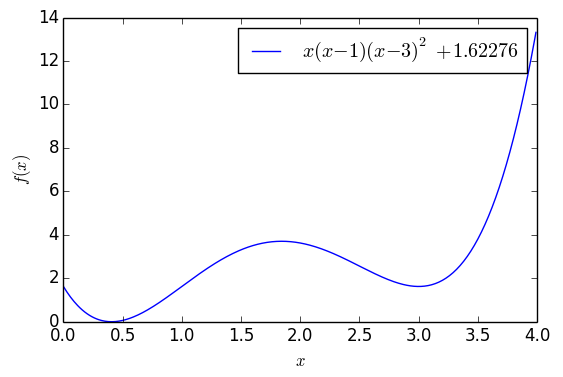 A univariate function with two local minima
This function has a global optimum somewhere around $x=0.41$, where the function value reaches 0, but there's also a suboptimal minimum near $x=3$. If we start from $x_0=4$ and use plain gradient descent, it will basically always converge to $x=3$. But if we use $\eqref{eq:me-gd-3}$, starting from the same $x_0=4$, after some oscillation it eventually converges near $x=0.41$:
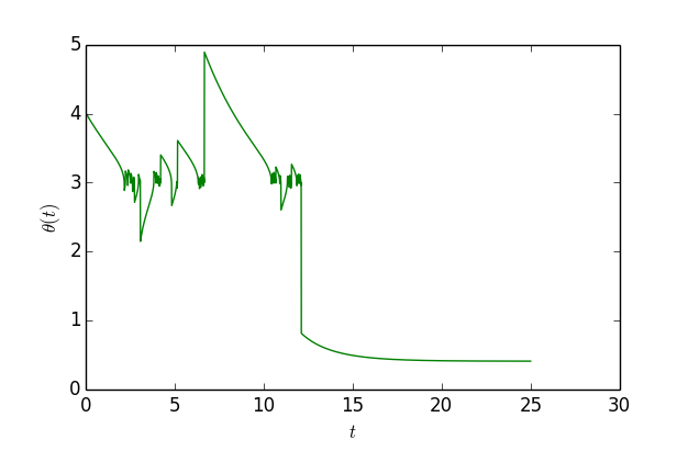 Simulated trajectory of the "homebrewed" gradient descent
You can see that at first it does hover around $x=3$, then after oscillating for a while it breaks free and ends up near $x=0.41$. Plotting code:
import numpy as np
import matplotlib.pyplot as plt

def f(x):
    return x * (x - 1) * (x - 3) * (x - 3) + 1.62276

def g(x):
    return -9 + 30 * x - 21 * x**2 + 4 * x**3

ts = [0]
xs = [4]
h = 0.01
H = 2500

for i in range(H):
    x = xs[-1]
    delta = -np.sign(g(x)) * min(abs(g(x)) / g(x)**2, 1000) * f(x)
    x += delta * h
    xs.append(x)
    ts.append(ts[-1] + h)

print f(xs[-1])
plt.figure()
plt.clf()
plt.plot(ts, xs, 'g')
plt.legend()
plt.xlabel('$t$')
plt.ylabel('$\\theta(t)$')
plt.show()
However, as nice as this looks, it turns out to have little practical value, because to really guarantee escaping all local optima, $M$ would need to be sufficiently large (so as to stay close enough to the original $\eqref{eq:me-gd-2}$), and the number of iterations would need to be large enough too. But if we could actually satisfy that condition, we might as well just add Gaussian noise to gradient descent ourselves—since, as we already showed in the first post, if the gradient noise is assumed Gaussian, then probabilistically speaking, we can always reach the global optimum (also requiring a sufficiently large number of iterations). So this seemingly elegant trick doesn't actually have much practical value.
(Note: I later learned, through further reading, that Polyak had already studied learning rates of the form in equation $\eqref{eq:me-gd}$ long ago. Searching for "Polyak step size" turns up plenty of related work, such as Revisiting the Polyak step size] and Generalized Polyak Step Size for First Order Optimization with Momentum].)
Summary
Well, after all this rambling and tinkering, another post is done. Personally, I find analyzing optimization algorithms from a dynamical-systems perspective to be a genuinely delightful exercise—it lets you appreciate the appeal of optimization algorithms in a relatively relaxed way, and even ties together knowledge from many different areas.
The usual way of understanding optimization algorithms starts from convex optimization, and then applies convex-optimization results somewhat loosely to the non-convex setting. We study convex optimization because "convexity" is such a powerful condition for many theoretical proofs—yet deep learning is non-convex almost everywhere. Given that we're already dealing with non-convexity, the main advantage of convex optimization—rigorous, complete proofs—no longer holds anyway. So I think it's better to approach the matter from a more relaxed angle. That more relaxed angle is dynamical systems, or equivalently, systems of ordinary differential equations.
In fact, this perspective has a lot of potential—including convergence analysis of GANs, and the much-discussed "Neural ODEs," both of which will eventually circle back to this very viewpoint. But that's a story for another time.
Translated automatically with claude-sonnet-5; all equations are reproduced verbatim from the source. Copyright remains with the original author.