Using Open-Source Human-Annotated Data to Enhance RoFormer-Sim

用开源的人工标注数据来增强RoFormer-Sim 苏剑林 · 2021-07-19 · Machine Learning language model generative model text generation

As many of you know, from SimBERT to SimBERTv2 (RoFormer-Sim), we've established a reasonably solid baseline model for Chinese text similarity tasks. However, SimBERT and RoFormer-Sim are, at their core, only "weakly supervised" models — similar to unsupervised models, we can't expect a purely weakly-supervised model to achieve results that perfectly match human intuition. So, in order to further improve RoFormer-Sim, we tried using some open-source annotated data to assist training. This post describes our exploration process.

Some readers might think: what's there to discuss about supervised training? Isn't it just direct training? Well, that's true in principle, but it's not actually as "obvious and straightforward" as it sounds — there are still some "landmines" to watch out for. So this post is also, in a sense, a simple "mine-clearing guide."

Recap

The author has noticed that, ever since SimBERT was released, the question readers ask most often is probably:

Why is the similarity between "I like Beijing" and "I don't like Beijing" so high? Don't they mean the opposite?

Especially after RoFormer-Sim was released, similar questions popped up almost once every week or two. Moreover, it's not just my own Kexue.fm discussion group — other NLP-related groups have also periodically raised similar questions, which suggests this confusion is widespread.

So how should we understand this?

First of all, the notion of "opposite meaning" isn't quite right. From a similarity standpoint, there's only "similar" and "dissimilar" — there's no such thing as "opposite." In principle, there are no two sentences that are absolutely unrelated to each other, so theoretically no pair of sentences has a similarity of exactly 0, let alone the ill-defined notion of "opposite." Quite the contrary — what we usually think of as "antonyms" are, objectively speaking, actually rather similar words. Take "like" and "dislike": they share a great deal in common — both are verbs, both describe emotional inclination, and their usage is quite similar. So how can we say these two words are "completely dissimilar" or even "opposite"? When we call them antonyms, we mean that they are opposed along some very narrow dimension — note, just one dimension, not all of them — which implies that this way of thinking is itself non-objective (if two words are similar along so many dimensions, and dissimilar along just one, and we still call them "antonyms," isn't that inherently a subjective judgment?).

By the same logic, from an objective standpoint, "I like Beijing" and "I don't like Beijing" are in fact quite similar, so it's entirely reasonable for the model to give them a high similarity score — a low score would actually be the unreasonable outcome. Of course, I'm not saying that "I like Beijing" and "I don't like Beijing" are similar in every context — they do differ along a specific dimension. But the issue is that what unsupervised and weakly-supervised learning produce are relatively objective results, whereas if we insist that "I like Beijing" and "I don't like Beijing" are dissimilar, that means we've subjectively singled out the particular dimension we want to compare, rather than considering all dimensions objectively. And since this is a subjective human judgment, we shouldn't expect unsupervised or weakly-supervised methods to learn it on their own — the best approach is to use annotated data for supervised learning.

So, to put it bluntly:

The model isn't wrong — people are. If people insist they're not wrong, then please tell the model it's wrong via supervised learning on annotated data.

Categorizing the Data

From the discussion above, we should now appreciate the necessity of supervised learning with annotated data. Not every problem can be solved via unsupervised or weakly-supervised methods; and if we insist on forcing an unsupervised or weakly-supervised solution, the cost may end up far exceeding that of simply annotating a handful of examples.

As for Chinese human-annotated data related to similarity, we've currently collected three types:

1. Binary type: This is the more common type, with the basic format "(sentence 1, sentence 2, whether similar)." The ATEC, BQ, LCQMC, and PAWSX datasets collected here are all of this type.
2. NLI type: NLI stands for Natural Language Inference, with samples in the format "(sentence 1, sentence 2, entailment/neutral/contradiction)." This can be viewed as a somewhat finer-grained similarity dataset. The Chinese NLI dataset currently available is translated from the English version; the link is at CNSD.
3. Scored type: This is the most fine-grained type of similarity corpus, with the format "(sentence 1, sentence 2, degree of similarity)," where the degree of similarity is usually on a finer-grained scale than a simple 0/1. The Chinese dataset currently available is STS-B, also translated from the corresponding English dataset.

Since the first two types have much larger volumes, for the sake of convenience we simply set a threshold to convert the third type (STS-B) into the format of the first type. So in the end there are two usable data formats: 1) binary classification of sentence pairs; 2) three-way classification of sentence pairs.

An Unexpected Turn

As mentioned at the start, even though this is supervised training, it's not quite as "obvious and straightforward" as it might seem — mainly because the choice of training scheme turned out to be somewhat unexpected. For simplicity, let's first illustrate this using binary-classification training samples.

Suppose the two sentences, after passing through the encoder, yield sentence vectors $u,v$. Since during retrieval we typically rank using their cosine value $\cos(u,v)=\frac{\langle u,v\rangle}{\Vert u\Vert \Vert v\Vert}$ as the similarity score, the natural idea is to design a loss function based on $\cos(u,v)$. Some readily conceivable options include:

\begin{equation}\begin{aligned} &t\cdot (\cos(u,v) - 1)^2 + (1 - t)\cdot \cos^2(u,v) \\ &t\cdot (\cos(u,v) - 1)^2 + (1 - t)\cdot (\cos(u,v) + 1)^2 \\ &t\cdot \max(0.9 - \cos(u,v), 0) + (1-t)\cdot \max(\cos(u,v) - 0.1, 0) \end{aligned}\end{equation}

where $t\in\{0,1\}$ is the label for the sentence pair. Roughly speaking, the above losses all aim to make $\cos(u,v)$ as large as possible for positive pairs, and $\cos(u,v)$ as small as possible for negative pairs.

However, in the author's experiments, this kind of training scheme — where training and prediction are consistent — actually performed worse than a scheme that originated in InferSent and was later adopted by Sentence-BERT, which at first glance appears inconsistent between training and prediction. Specifically, Sentence-BERT concatenates $u,v,|u-v|$ (where $|u-v|$ denotes the vector obtained by taking the absolute value of each element of $u-v$) as features, followed by a fully connected layer for binary classification (or three-way classification, in the case of NLI datasets).

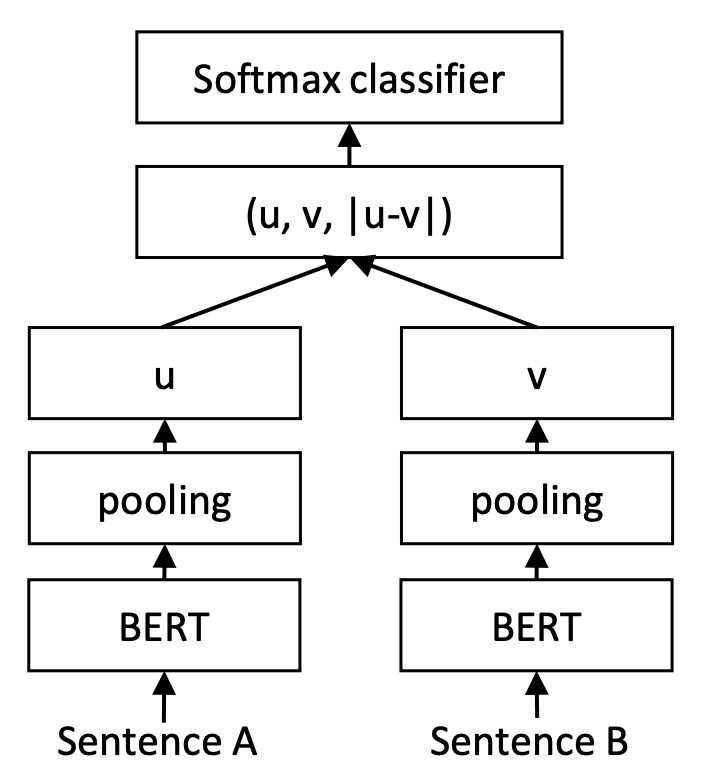Sentence-BERT during training 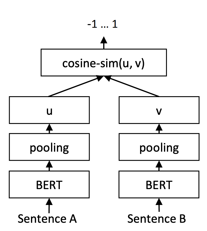Sentence-BERT during prediction

Of course, this is only the training scheme; at inference time, we still take out the sentence vectors and use cosine similarity for retrieval. Seen this way, the scheme used by InferSent and Sentence-BERT is, in fact, one where training and prediction are inconsistent — training doesn't directly involve $\cos(u,v)$, yet at prediction time we can use $\cos(u,v)$ for retrieval, and it still performs quite well. This can't help but be a bit surprising.

Reasoning It Out on My Own

The author was, frankly, quite puzzled by this. I noticed that the Sentence-BERT paper also compares different ways of combining features for the final result, showing that concatenating $u,v,|u-v|$ gives the best performance — if you keep only part of these components, performance drops noticeably, as shown in the table below.

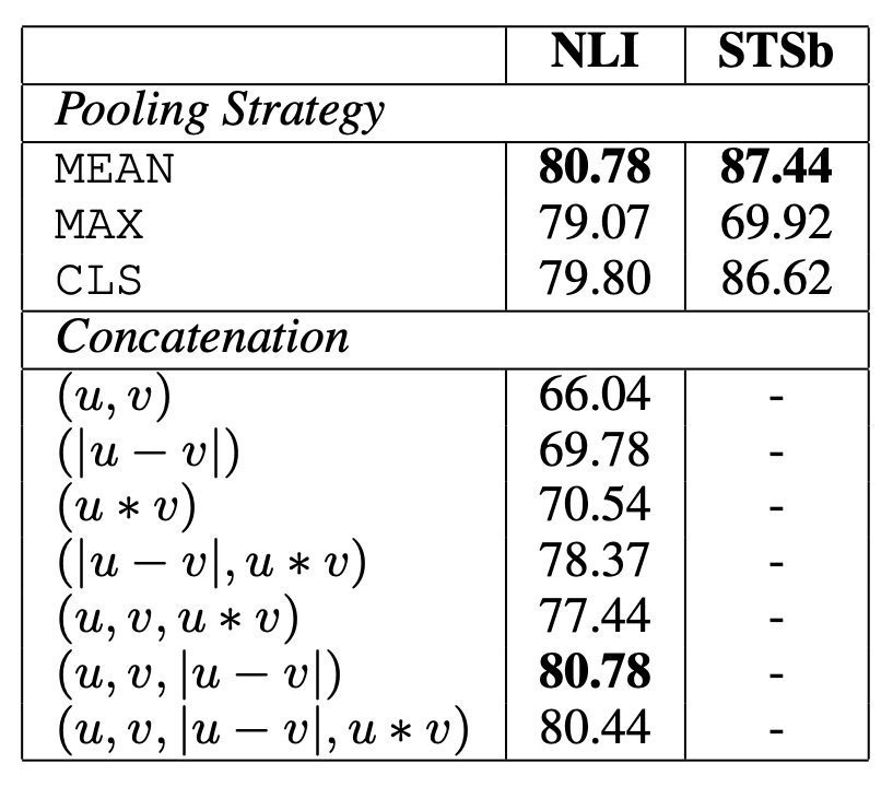Experimental results for different concatenated features

Inspired by this table, the author — working things out on my own, so to speak — came up with an explanation. First, we know that people are quite "picky," especially when it comes to similarity tasks: we tend to consider only fairly strict similarity as "similar," yet our training data usually isn't that precise. On the one hand, the annotations themselves may contain noise; on the other hand, for certain sentence pairs, annotators may label them as positive simply because they share the same topic (rather than the same semantics). In other words, annotated data is usually not as strict as we would like, and if we directly use the annotation results to learn our ranking metric, this can actually introduce unexpected biases.

Looking back at the approach of concatenating $u,v,|u-v|$ followed by a fully connected layer, its scoring function is essentially

\begin{equation}s = \langle u, w_1\rangle + \langle v, w_2\rangle + \langle |u-v|, w_3\rangle\end{equation}

Here $w_1,w_2,w_3$ is the corresponding parameter vector. The first two terms give a score of $\langle u, w_1\rangle + \langle v, w_2\rangle$; if this is large, it doesn't necessarily mean $u,v$ are close, and likewise, if it's small, it doesn't necessarily mean $u,v$ are far apart — its role is more like a "topic classification" model, used to determine whether the topics of $u,v$ are consistent. As for the third term, we know that $|u-v|=0\Leftrightarrow u=v$, so this third term is genuinely capable of judging how close the two vectors are — it perhaps represents true "semantic similarity."

Putting this together, we can say that the approach of concatenating $u,v,|u-v|$ and then applying a fully connected layer incorporates both a score for whether the topics of the two sentences match and a score for their semantic similarity. It separates "topic" from "semantics," which increases the model's tolerance for noisy data, and as a result, the vectors ultimately learned better reflect a purer, more precise notion of "semantics."

Having Your Cake and Eating It Too

Through the Sentence-BERT scheme, by using open-source similarity datasets, we can learn a fairly effective sentence-vector model — that is, a retrieval model — such that extracting features with it and using cosine similarity as the metric gives good results. But the problem is that SimBERT and RoFormer-Sim were never meant to be pure retrieval models. What we want is to "have our cake and eat it too" — both good retrieval performance and the ability to generate similar sentences.

To achieve this, after training a Sentence-BERT model as described above, we distill its retrieval performance into RoFormer-Sim using the approach introduced in SimBERTv2 Is Here! The RoFormer-Sim Model That Combines Retrieval and Generation, thereby improving the retrieval model's performance while retaining the ability to generate similar sentences. Moreover, distillation between models of the same size often gives a bit of an extra boost, so the retrieval performance of our distilled RoFormer-Sim actually turns out to be even better than the directly-trained Sentence-BERT.

Demonstration

We've open-sourced the RoFormer-Sim trained with annotated data as follows (the weight files with "-ft" in their names):

https://github.com/ZhuiyiTechnology/roformer-sim

Below are the test results (on the test sets) for several tasks from Which Unsupervised Semantic Similarity Method Is Best? A Fairly Comprehensive Evaluation:

$$\begin{array}{c|ccccc} \hline & \text{ATEC} & \text{BQ} & \text{LCQMC} & \text{PAWSX} & \text{STS-B} \\ \hline \text{RoFormer-Sim} & 39.27 & 48.31 & 72.30 & 6.70 & 71.75 \\ \text{RoFormer-Sim-FT} & 51.71 & 73.48 & 79.56 & 62.84 & 78.28 \\ \hline \text{RoFormer-Sim-small} & 37.08 & 46.83 & 71.27 & 5.8 & 71.29 \\ \text{RoFormer-Sim-FT-small} & 51.21 & 73.09 & 78.88 & 56.41 & 76.33 \\ \hline \end{array}$$

We can see a clear improvement, and the small version also performs quite respectably. Of course, since this involves supervised training, an improvement is to be expected, so this comparison table isn't hugely meaningful in itself. But for users, all that matters is having a ready-to-use model — who cares how it was made, right? What readers probably care more about is whether this new model resolves the previous retrieval model's "pain point" — for instance, can it widen the gap between "I like Beijing" and "I don't like Beijing"? Let's look at a few examples below (base version; the small version gives nearly identical results):

similarity(u'今天天气不错', u'今天天气很好')
0.9769838
similarity(u'今天天气不错', u'今天天气不好')
0.62359834
similarity(u'我喜欢北京', u'我很喜欢北京')
0.9921096
similarity(u'我喜欢北京', u'我不喜欢北京')
0.5291042
similarity(u'电影不错', u'电影很好')
0.96764225
similarity(u'电影不错', u'电影不好')
0.6312722
similarity(u'红色的苹果', u'绿色的苹果')
0.6974633
similarity(u'给我推荐一款红色的车', u'给我推荐一款黑色的车')
0.7191832
similarity(u'给我推荐一款红色的车', u'推荐一辆红车')
0.9866457
similarity(u'给我推荐一款红色的车', u'麻烦来一辆红车')
0.9460306

From these examples, we can see that after supervised training, the model does produce similarity scores that better match common-sense human intuition — for instance, adding a negation word noticeably lowers the similarity score. Upon comparison, we found this effect is mainly attributable to the NLI dataset. Also, the model has become more sensitive to color words like "red" and "black," and, especially in the last three examples, its ranking of retrieval results now aligns much better with typical intent-recognition scenarios.

Summary

This post described our process of using annotated data to enhance RoFormer-Sim, and we've open-sourced the resulting trained model, giving the Chinese similarity-modeling community a better-performing, open-source baseline to use.