Which unsupervised semantic similarity method is best? We ran a fairly comprehensive evaluation

无监督语义相似度哪家强？我们做了个比较全面的评测 苏剑林 · 2021-04-11 · Machine Learning language model semantics semantic similarity

Back in January, I wrote You Probably Don't Need BERT-flow: A Linear Transformation Rivals BERT-flow, pointing out that BERT-flow, the SOTA model for unsupervised semantic similarity, can actually be matched by a simple linear transformation (a whitening operation, BERT-whitening). Since then, we've further refined the experimental results and turned them into a paper, Whitening Sentence Representations for Better Semantics and Faster Retrieval. This post gives a basic walkthrough of that paper's content, and supplements it with additional evaluations on 5 Chinese semantic similarity tasks, comprising more than 600 experimental results.

GitHub link: https://github.com/bojone/BERT-whitening

Method Overview

The idea behind BERT-whitening is simple: after obtaining the sentence vector $\{x_i\}_{i=1}^N$ for each sentence, we whiten these matrices (i.e., apply PCA) so that each dimension has zero mean and the covariance matrix becomes the identity, and then keep the top $k$ principal components. The pipeline is shown below:

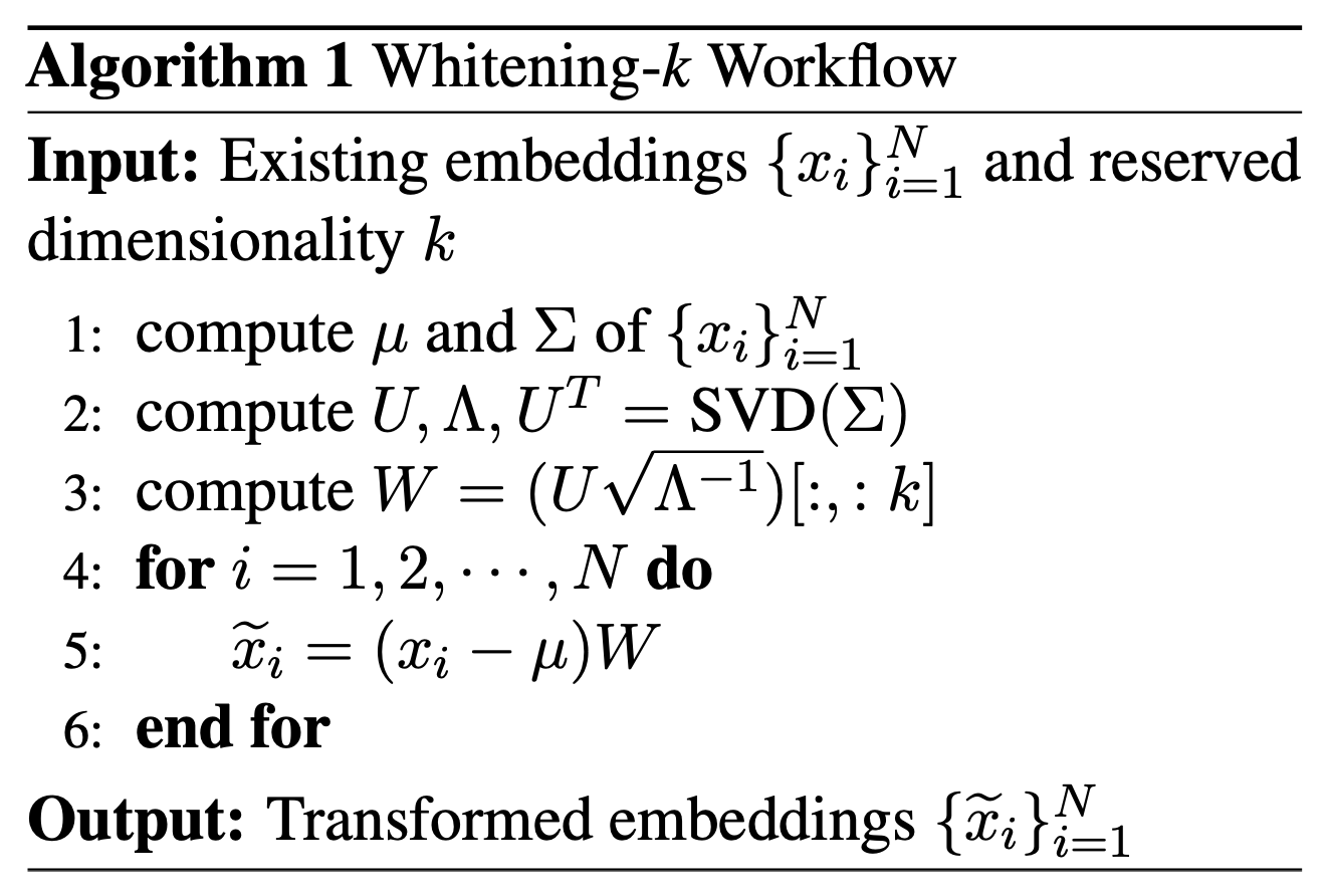The basic pipeline of BERT-whitening]more

Theoretically, of course, we can also view BERT-whitening as the simplest possible implementation of BERT-flow, and as pointed out in the earlier post, this simple implementation is already enough to rival, and sometimes surpass, the general BERT-flow model. At the same time, since whitening also ranks feature importance as part of the transformation, we can reduce the dimensionality of sentence vectors to speed up retrieval. The experimental results show that in most tasks, dimensionality reduction not only doesn't hurt performance, but can actually improve it.

English Tasks

Let's first look at the test results of BERT-whitening on English tasks, covering three tables in total, which essentially provide a rigorous side-by-side comparison with BERT-flow.

Purely Unsupervised

The first table presents results in the fully unsupervised setting, i.e., directly extracting sentence vectors from a pretrained BERT with no additional supervision. In the BERT-flow paper, we already confirmed that, without any post-processing, the best pooling method for extracting sentence vectors from BERT is averaging all token vectors across the first and last layers, i.e., first-last-avg (the BERT-flow paper mistakenly identified this as averaging the last two layers, labeling it last2avg, when it's actually the first and last layers). So all the results below use first-last-avg as the baseline on top of which flow or whitening is applied.

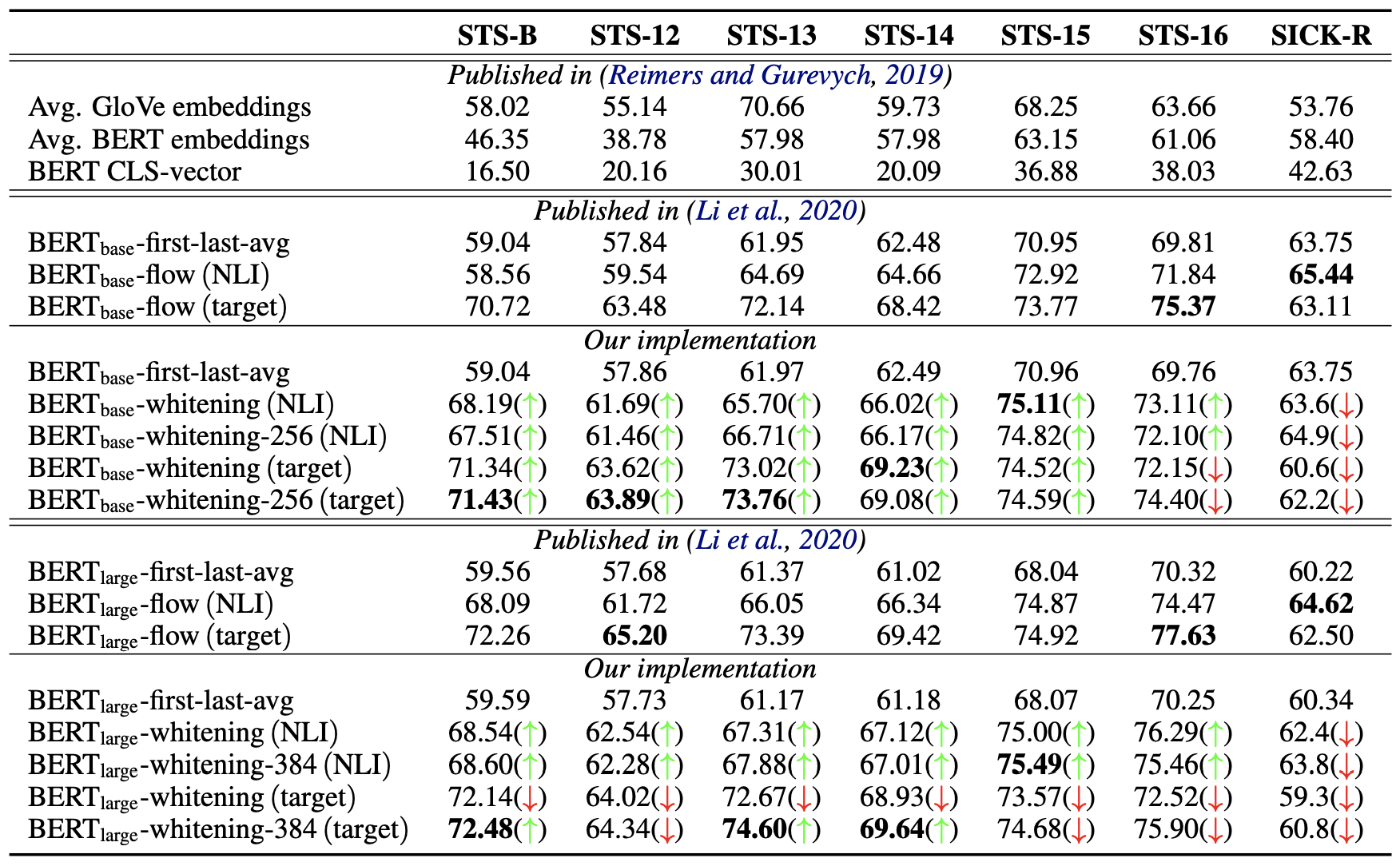Evaluation results for purely unsupervised semantic matching on English tasks]

NLI-Supervised

The second table shows results using sentence vectors extracted from Sentence-BERT (SBERT) models fine-tuned on NLI datasets. Here too, first-last-avg is the best pooling method, so the baseline for both flow and whitening is the sentence vector produced by first-last-avg. The NLI dataset is a natural language inference dataset, which is similar to but not the same as semantic similarity; it can serve as supervised pretraining for semantic similarity tasks, but since it doesn't directly use semantic similarity data, it's still considered unsupervised relative to the semantic similarity task itself.

Evaluation results for BERT-NLI-based semantic matching on English tasks]

Dimensionality vs. Performance

In both tables, the bolded entries are the best results; a green arrow $\color{green}{\uparrow}$ means that BERT-whitening outperforms BERT-flow under the same setting, while a red arrow $\color{red}{\downarrow}$ means the opposite—so the more green arrows, the better BERT-whitening performs overall. The numbers after "whitening", like 256 or 384, denote the retained dimensionality after reduction. From these two tables we can see that BERT-whitening generally outperforms BERT-flow, achieving SOTA on most tasks, and in most cases, dimensionality reduction further boosts performance.

To further confirm the effect of dimensionality reduction, we plotted the following dimensionality-vs-performance curves:

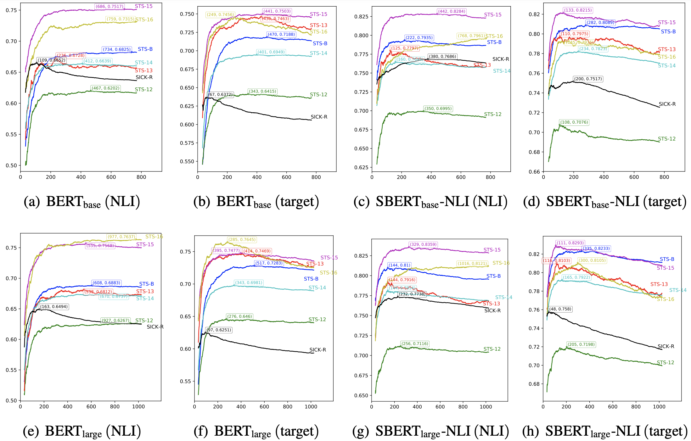"Dimensionality vs. performance" plots for each English task, with the dimensionality corresponding to the best performance marked. It's clear that for every task, dimensionality reduction can bring some improvement.]

The figure above shows, for each model on each task, how the evaluation metric changes with the retained dimensionality after whitening. As we can see, for every task the optimum is never achieved at full dimensionality, meaning that dimensionality reduction can always yield some improvement. In fact, quite a few tasks can be reduced to 1/8 of the original dimensionality or even further while maintaining or even improving performance—this really highlights the practical engineering value of BERT-whitening, since reduced dimensionality translates directly into much faster retrieval.

Chinese Tasks

In keeping with the principle that "a model that hasn't been tested on Chinese has no soul," I compiled several Chinese semantic similarity datasets and evaluated combinations of different Chinese pretrained models, pooling methods, and whitening (or not). The results are summarized below for everyone's reference.

Evaluation Setup

This evaluation covers 11 models, 5 datasets, and 4 pooling methods, with each combination compared across 3 post-processing strategies: "no whitening," "whitening," and "whitening plus dimensionality reduction." That gives close to

$$11\times 5\times 4\times 3 = 660$$

experimental results in total—fairly comprehensive. I say "close to" because some pooling methods aren't applicable to certain models, so the actual count falls a bit short of 660. Since BERT-flow is significantly more computationally expensive than BERT-whitening, we didn't reproduce a BERT-flow comparison here; but based on the English task results, BERT-whitening and BERT-flow tend to perform similarly, with BERT-whitening usually slightly ahead, so the whitening results here should be reasonably representative.

The evaluation metric is the same as in the English tasks: Spearman's correlation coefficient, which is an AUC-like ranking metric that depends only on the ordering of predicted scores and not on any threshold, making it well suited for this kind of evaluation. We didn't use the more familiar accuracy metric, partly because accuracy depends on a specific threshold, and partly because the labels in the STS-B dataset are numbers from 1 to 5 rather than 0/1 labels, so accuracy isn't even well-defined there. Hence we consistently use the Spearman correlation. If readers insist on an accuracy-based intuition, a rough approximation would be "accuracy ≈ 0.5 + spearman / 2."

The 11 models are as follows:

BERT: Google's open-sourced Chinese BERT base, link;
RoBERTa: HIT's open-sourced roberta_wwm_ext base version, link;
NEZHA: Huawei's open-sourced BERT base with relative position encoding (wwm), link;
WoBERT: word-level BERT, using the Plus version here, link;
RoFormer: BERT with a novel positional encoding, link;
BERTlarge: Tencent UER's open-sourced BERT large version, link;
RoBERTalarge: HIT's open-sourced roberta_wwm_ext large version, link;
NEZHA-large: Huawei's open-sourced BERT large with relative position encoding (wwm), link;
SimBERT: BERT base trained on similar-sentence pairs, link;
SimBERTsmall: BERT small trained on similar-sentence pairs, link;
SimBERTtiny: BERT tiny trained on similar-sentence pairs, link.

The 5 tasks are as follows:

ATEC: the ATEC semantic similarity competition dataset, from the financial customer-service domain; the original competition link is dead, current data available at link;
BQ: HIT's BQ Corpus dataset, question matching in the banking/finance domain, details at link;
LCQMC: HIT's LCQMC dataset, question matching covering multiple domains, details at link;
PAWSX: a dataset released by Google (link) containing multilingual paraphrase and non-paraphrase pairs, i.e., determining whether a pair of sentences share the same meaning. Its distinguishing feature is a high degree of lexical overlap, making it a relatively hard task for unsupervised methods; only the Chinese portion is retained here;
STS-B: measuring the correlation between two sentences; the original dataset is in English, and the Chinese version was produced via translation plus some manual correction, source link.

The 4 pooling methods are as follows:

P1: take the [CLS] vector from the encoder's last layer;
P2: take the vector output by the Pooler (which BERT uses for the NSP task)—this differs from P1 by an extra linear transformation;
P3: average all vectors from the encoder's last layer;
P4: average all vectors across the encoder's first and last layers.

Summary of Results

All experimental results are summarized in the following three tables. Each entry in the tables takes the form $a / b / c$, representing, for that task under that model: a score of $a$ with "no whitening," a score of $b$ with "whitening," and a score of $c$ with "whitening plus appropriate dimensionality reduction." If $b\geq a$, then $b$ is shown in green, otherwise in red; if $c\geq a$, then $c$ is shown in green, otherwise in red. "Appropriate dimensionality reduction" here means reducing to 256 dimensions for base models, 384 dimensions for large models, and 128 dimensions for the tiny and small models.

The first table compares 6 of the 11 models, all base-sized versions. Note that WoBERT and RoFormer don't have an NSP task, so there are no P2 weights and P2 can't be tested for them:

$$\small{\begin{array}{l|ccccc} \hline & \text{ATEC} & \text{BQ} & \text{LCQMC} & \text{PAWSX} & \text{STS-B} \\ \hline \text{BERT-P1} & 16.59 / \color{green}{20.61} / \color{green}{25.58} & 29.35 / \color{red}{25.76} / \color{green}{34.66} & 41.71 / \color{green}{48.92} / \color{green}{49.18} & 15.15 / \color{green}{17.03} / \color{green}{15.98} & 34.65 / \color{green}{61.19} / \color{green}{60.07} \\ \text{BERT-P2} & 9.46 / \color{green}{22.16} / \color{green}{25.13} & 16.97 / \color{green}{18.97} / \color{green}{33.99} & 28.42 / \color{green}{49.61} / \color{green}{49.59} & 13.93 / \color{green}{16.08} / \color{green}{16.19} & 21.66 / \color{green}{60.75} / \color{green}{60.13} \\ \text{BERT-P3} & 20.79 / \color{red}{18.27} / \color{green}{28.98} & 33.08 / \color{red}{22.58} / \color{green}{38.62} & 59.22 / \color{green}{60.12} / \color{green}{62.00} & 16.68 / \color{green}{18.37} / \color{green}{17.38} & 57.48 / \color{green}{63.97} / \color{green}{68.27} \\ \text{BERT-P4} & 24.51 / \color{green}{27.00} / \color{green}{27.91} & 38.81 / \color{red}{32.29} / \color{red}{37.67} & 64.75 / \color{green}{64.75} / \color{green}{65.65} & 15.12 / \color{green}{17.80} / \color{green}{15.34} & 61.66 / \color{green}{69.45} / \color{green}{69.37} \\ \hline \text{RoBERTa-P1} & 24.61 / \color{green}{29.59} / \color{green}{29.49} & 40.54 / \color{red}{28.95} / \color{red}{38.35} & 70.55 / \color{green}{70.82} / \color{red}{68.84} & 16.23 / \color{green}{17.99} / \color{green}{16.87} & 66.91 / \color{green}{69.19} / \color{green}{71.16} \\ \text{RoBERTa-P2} & 20.61 / \color{green}{28.91} / \color{green}{29.49} & 31.14 / \color{red}{27.48} / \color{green}{38.46} & 65.43 / \color{green}{70.62} / \color{green}{68.76} & 15.71 / \color{green}{17.30} / \color{green}{17.01} & 59.50 / \color{green}{70.77} / \color{green}{71.16} \\ \text{RoBERTa-P3} & 26.94 / \color{green}{29.94} / \color{green}{30.57} & 40.71 / \color{red}{30.95} / \color{red}{39.89} & 66.80 / \color{green}{68.00} / \color{green}{67.30} & 16.08 / \color{green}{19.01} / \color{green}{16.79} & 61.67 / \color{green}{66.19} / \color{green}{69.36} \\ \text{RoBERTa-P4} & 27.94 / \color{green}{28.33} / \color{green}{29.06} & 43.09 / \color{red}{33.49} / \color{red}{38.83} & 68.43 / \color{red}{67.86} / \color{red}{68.36} & 15.02 / \color{green}{17.91} / \color{green}{15.26} & 64.09 / \color{green}{69.74} / \color{green}{70.09} \\ \hline \text{NEZHA-P1} & 17.39 / \color{green}{18.83} / \color{green}{24.97} & 29.63 / \color{red}{21.94} / \color{green}{33.65} & 40.60 / \color{green}{50.52} / \color{green}{46.57} & 14.90 / \color{green}{18.15} / \color{green}{16.69} & 35.84 / \color{green}{60.84} / \color{green}{58.98} \\ \text{NEZHA-P2} & 10.96 / \color{green}{23.08} / \color{green}{24.21} & 17.38 / \color{green}{28.81} / \color{green}{32.21} & 22.66 / \color{green}{49.12} / \color{green}{47.03} & 13.45 / \color{green}{18.05} / \color{green}{17.15} & 21.16 / \color{green}{60.11} / \color{green}{58.68} \\ \text{NEZHA-P3} & 23.70 / \color{red}{21.93} / \color{green}{28.65} & 35.44 / \color{red}{22.44} / \color{green}{37.95} & 60.94 / \color{green}{62.10} / \color{green}{62.50} & 18.35 / \color{green}{21.72} / \color{green}{18.78} & 60.35 / \color{green}{68.57} / \color{green}{68.97} \\ \text{NEZHA-P4} & 27.72 / \color{red}{25.31} / \color{red}{26.18} & 44.18 / \color{red}{31.47} / \color{red}{36.02} & 65.16 / \color{green}{66.68} / \color{green}{66.54} & 13.98 / \color{green}{16.66} / \color{green}{14.02} & 61.94 / \color{green}{69.55} / \color{green}{69.14} \\ \hline \text{WoBERT-P1} & 23.88 / \color{red}{22.45} / \color{green}{27.88} & 43.08 / \color{red}{32.52} / \color{red}{37.54} & 68.56 / \color{red}{67.89} / \color{red}{65.80} & 18.15 / \color{green}{19.92} / \color{green}{18.73} & 64.12 / \color{green}{66.53} / \color{green}{69.03} \\ \text{WoBERT-P2} & \text{-} & \text{-} & \text{-} & \text{-} & \text{-} \\ \text{WoBERT-P3} & 24.62 / \color{red}{22.74} / \color{green}{29.01} & 40.64 / \color{red}{28.12} / \color{red}{38.82} & 64.89 / \color{green}{65.22} / \color{green}{65.14} & 16.83 / \color{green}{20.56} / \color{green}{17.87} & 59.43 / \color{green}{66.57} / \color{green}{67.76} \\ \text{WoBERT-P4} & 25.97 / \color{green}{27.24} / \color{green}{28.38} & 42.37 / \color{red}{32.34} / \color{red}{38.06} & 66.53 / \color{red}{65.62} / \color{red}{66.36} & 15.54 / \color{green}{18.85} / \color{green}{15.98} & 61.37 / \color{green}{68.11} / \color{green}{68.42} \\ \hline \text{RoFormer-P1} & 24.29 / \color{green}{26.04} / \color{green}{28.20} & 41.91 / \color{red}{28.13} / \color{red}{38.21} & 64.87 / \color{red}{60.92} / \color{red}{60.83} & 20.15 / \color{green}{23.08} / \color{green}{21.30} & 59.91 / \color{green}{66.96} / \color{green}{66.86} \\ \text{RoFormer-P2} & \text{-} & \text{-} & \text{-} & \text{-} & \text{-} \\ \text{RoFormer-P3} & 24.09 / \color{green}{28.51} / \color{green}{29.37} & 39.09 / \color{red}{34.92} / \color{red}{39.05} & 63.55 / \color{green}{63.85} / \color{green}{63.58} & 16.53 / \color{green}{18.43} / \color{green}{17.52} & 58.98 / \color{red}{55.30} / \color{green}{67.32} \\ \text{RoFormer-P4} & 25.92 / \color{green}{27.38} / \color{green}{28.37} & 41.75 / \color{red}{32.36} / \color{red}{38.05} & 66.18 / \color{red}{65.45} / \color{red}{65.63} & 15.30 / \color{green}{18.36} / \color{green}{15.69} & 61.40 / \color{green}{68.02} / \color{green}{68.27} \\ \hline \text{SimBERT-P1} & 38.50 / \color{red}{23.64} / \color{red}{30.79} & 48.54 / \color{red}{31.78} / \color{red}{40.01} & 76.23 / \color{red}{75.05} / \color{red}{74.50} & 15.10 / \color{green}{18.49} / \color{green}{15.64} & 74.14 / \color{red}{73.37} / \color{green}{75.29} \\ \text{SimBERT-P2} & 38.93 / \color{red}{27.06} / \color{red}{30.79} & 49.93 / \color{red}{35.38} / \color{red}{40.14} & 75.56 / \color{red}{73.45} / \color{red}{74.39} & 14.52 / \color{green}{18.51} / \color{green}{15.74} & 73.18 / \color{green}{73.43} / \color{green}{75.12} \\ \text{SimBERT-P3} & 36.50 / \color{red}{31.32} / \color{red}{31.24} & 45.78 / \color{red}{29.17} / \color{red}{40.98} & 74.42 / \color{red}{73.79} / \color{red}{73.43} & 15.33 / \color{green}{18.39} / \color{green}{15.87} & 67.31 / \color{green}{70.70} / \color{green}{72.00} \\ \text{SimBERT-P4} & 33.53 / \color{red}{29.04} / \color{red}{28.78} & 45.28 / \color{red}{34.70} / \color{red}{39.00} & 73.20 / \color{red}{71.22} / \color{red}{72.09} & 14.16 / \color{green}{17.32} / \color{green}{14.39} & 66.98 / \color{green}{70.55} / \color{green}{71.43} \\ \hline \end{array}}$$

The second table compares the 3 large-sized models:

$$\small{\begin{array}{l|ccccc} \hline & \text{ATEC} & \text{BQ} & \text{LCQMC} & \text{PAWSX} & \text{STS-B} \\ \hline \text{BERT}_{\text{large}}\text{-P1} & 13.15 / \color{green}{22.42} / \color{green}{24.32} & 19.81 / \color{red}{17.61} / \color{green}{31.09} & 23.45 / \color{green}{44.31} / \color{green}{41.32} & 16.88 / \color{green}{19.37} / \color{green}{19.87} & 25.93 / \color{green}{52.70} / \color{green}{56.74} \\ \text{BERT}_{\text{large}}\text{-P2} & 8.16 / \color{green}{16.57} / \color{green}{24.34} & 9.43 / \color{green}{18.23} / \color{green}{30.91} & 16.66 / \color{green}{39.50} / \color{green}{41.40} & 14.72 / \color{green}{20.00} / \color{green}{19.92} & 15.82 / \color{green}{56.79} / \color{green}{56.73} \\ \text{BERT}_{\text{large}}\text{-P3} & 24.31 / \color{red}{18.25} / \color{green}{30.24} & 35.87 / \color{red}{32.56} / \color{green}{37.51} & 59.29 / \color{green}{65.06} / \color{green}{63.78} & 16.94 / \color{green}{20.01} / \color{green}{18.62} & 60.22 / \color{green}{68.07} / \color{green}{68.87} \\ \text{BERT}_{\text{large}}\text{-P4} & 25.62 / \color{green}{27.64} / \color{green}{28.15} & 38.45 / \color{red}{31.30} / \color{red}{36.47} & 65.43 / \color{green}{66.54} / \color{green}{67.02} & 15.33 / \color{green}{19.06} / \color{green}{15.95} & 62.02 / \color{green}{69.74} / \color{green}{69.99} \\ \hline \text{RoBERTa}_{\text{large}}\text{-P1} & 19.32 / \color{red}{15.90} / \color{green}{29.32} & 34.21 / \color{red}{23.16} / \color{green}{37.11} & 64.89 / \color{green}{67.05} / \color{green}{66.49} & 17.78 / \color{green}{20.66} / \color{green}{19.73} & 60.16 / \color{green}{69.46} / \color{green}{70.44} \\ \text{RoBERTa}_{\text{large}}\text{-P2} & 19.32 / \color{green}{22.16} / \color{green}{29.23} & 34.33 / \color{red}{33.22} / \color{green}{37.10} & 65.00 / \color{green}{67.12} / \color{green}{66.50} & 17.77 / \color{green}{18.90} / \color{green}{19.79} & 60.09 / \color{green}{61.35} / \color{green}{70.32} \\ \text{RoBERTa}_{\text{large}}\text{-P3} & 24.83 / \color{red}{21.05} / \color{green}{30.85} & 39.23 / \color{red}{26.85} / \color{red}{38.39} & 66.86 / \color{green}{68.62} / \color{green}{67.25} & 17.67 / \color{green}{20.06} / \color{green}{19.09} & 62.98 / \color{red}{55.75} / \color{green}{69.72} \\ \text{RoBERTa}_{\text{large}}\text{-P4} & 25.69 / \color{green}{28.19} / \color{green}{28.39} & 40.18 / \color{red}{32.06} / \color{red}{36.91} & 68.58 / \color{green}{68.74} / \color{green}{68.71} & 16.01 / \color{green}{19.87} / \color{green}{16.50} & 63.75 / \color{green}{70.08} / \color{green}{70.39} \\ \hline \text{NEZHA}_{\text{large}}\text{-P1} & 18.91 / \color{green}{24.98} / \color{green}{25.68} & 30.39 / \color{red}{29.30} / \color{green}{33.29} & 41.68 / \color{green}{52.42} / \color{green}{49.80} & 18.89 / \color{green}{23.31} / \color{green}{21.74} & 39.04 / \color{green}{60.36} / \color{green}{61.13} \\ \text{NEZHA}_{\text{large}}\text{-P2} & 7.92 / \color{green}{21.60} / \color{green}{25.33} & 12.03 / \color{green}{24.63} / \color{green}{33.22} & 12.33 / \color{green}{52.40} / \color{green}{49.68} & 16.26 / \color{green}{23.11} / \color{green}{21.95} & 16.59 / \color{green}{57.70} / \color{green}{60.82} \\ \text{NEZHA}_{\text{large}}\text{-P3} & 22.74 / \color{green}{25.63} / \color{green}{27.48} & 36.48 / \color{red}{22.33} / \color{red}{35.47} & 59.65 / \color{green}{59.90} / \color{green}{59.94} & 18.09 / \color{green}{23.12} / \color{green}{19.71} & 59.66 / \color{green}{67.80} / \color{green}{68.55} \\ \text{NEZHA}_{\text{large}}\text{-P4} & 27.45 / \color{red}{24.83} / \color{red}{24.90} & 44.33 / \color{red}{29.73} / \color{red}{34.05} & 66.19 / \color{green}{66.89} / \color{green}{67.88} & 13.74 / \color{green}{16.66} / \color{green}{13.95} & 62.91 / \color{green}{69.87} / \color{green}{69.71} \\ \hline \end{array}}$$

The third table compares SimBERT models of different sizes against each other:

$$\small{\begin{array}{l|ccccc} \hline & \text{ATEC} & \text{BQ} & \text{LCQMC} & \text{PAWSX} & \text{STS-B} \\ \hline \text{SimBERT}\text{-P1} & 38.50 / \color{red}{23.64} / \color{red}{30.79} & 48.54 / \color{red}{31.78} / \color{red}{40.01} & 76.23 / \color{red}{75.05} / \color{red}{74.50} & 15.10 / \color{green}{18.49} / \color{green}{15.64} & 74.14 / \color{red}{73.37} / \color{green}{75.29} \\ \text{SimBERT}\text{-P2} & 38.93 / \color{red}{27.06} / \color{red}{30.79} & 49.93 / \color{red}{35.38} / \color{red}{40.14} & 75.56 / \color{red}{73.45} / \color{red}{74.39} & 14.52 / \color{green}{18.51} / \color{green}{15.74} & 73.18 / \color{green}{73.43} / \color{green}{75.12} \\ \text{SimBERT}\text{-P3} & 36.50 / \color{red}{31.32} / \color{red}{31.24} & 45.78 / \color{red}{29.17} / \color{red}{40.98} & 74.42 / \color{red}{73.79} / \color{red}{73.43} & 15.33 / \color{green}{18.39} / \color{green}{15.87} & 67.31 / \color{green}{70.70} / \color{green}{72.00} \\ \text{SimBERT}\text{-P4} & 33.53 / \color{red}{29.04} / \color{red}{28.78} & 45.28 / \color{red}{34.70} / \color{red}{39.00} & 73.20 / \color{red}{71.22} / \color{red}{72.09} & 14.16 / \color{green}{17.32} / \color{green}{14.39} & 66.98 / \color{green}{70.55} / \color{green}{71.43} \\ \hline \text{SimBERT}_{\text{small}}\text{-P1} & 30.68 / \color{red}{27.56} / \color{red}{29.07} & 43.41 / \color{red}{30.89} / \color{red}{39.78} & 74.73 / \color{red}{73.21} / \color{red}{73.50} & 15.89 / \color{green}{17.96} / \color{green}{16.75} & 70.54 / \color{green}{71.39} / \color{green}{72.14} \\ \text{SimBERT}_{\text{small}}\text{-P2} & 31.00 / \color{red}{29.14} / \color{red}{29.11} & 43.76 / \color{red}{36.86} / \color{red}{39.84} & 74.21 / \color{red}{73.14} / \color{red}{73.67} & 16.17 / \color{green}{18.12} / \color{green}{16.81} & 70.10 / \color{green}{71.40} / \color{green}{72.28} \\ \text{SimBERT}_{\text{small}}\text{-P3} & 30.03 / \color{red}{21.24} / \color{red}{29.30} & 43.72 / \color{red}{31.69} / \color{red}{40.81} & 72.12 / \color{red}{70.27} / \color{red}{70.52} & 16.93 / \color{green}{21.68} / \color{green}{18.75} & 66.55 / \color{red}{66.11} / \color{green}{69.19} \\ \text{SimBERT}_{\text{small}}\text{-P4} & 29.52 / \color{red}{28.41} / \color{red}{28.57} & 43.52 / \color{red}{36.56} / \color{red}{40.49} & 70.33 / \color{red}{68.75} / \color{red}{69.01} & 15.39 / \color{green}{21.57} / \color{green}{16.34} & 64.73 / \color{green}{68.12} / \color{green}{68.24} \\ \hline \text{SimBERT}_{\text{tiny}}\text{-P1} & 30.51 / \color{red}{24.67} / \color{red}{27.98} & 44.25 / \color{red}{31.75} / \color{red}{39.42} & 74.27 / \color{red}{72.25} / \color{red}{73.24} & 16.01 / \color{green}{18.07} / \color{green}{17.07} & 70.11 / \color{red}{66.39} / \color{green}{71.92} \\ \text{SimBERT}_{\text{tiny}}\text{-P2} & 30.01 / \color{red}{27.66} / \color{red}{27.92} & 44.47 / \color{red}{37.33} / \color{red}{39.39} & 73.98 / \color{red}{72.31} / \color{red}{73.31} & 16.55 / \color{green}{18.15} / \color{green}{17.14} & 70.35 / \color{green}{70.88} / \color{green}{72.04} \\ \text{SimBERT}_{\text{tiny}}\text{-P3} & 28.47 / \color{red}{19.68} / \color{green}{28.60} & 42.04 / \color{red}{29.49} / \color{red}{40.59} & 69.16 / \color{red}{66.99} / \color{red}{67.74} & 16.18 / \color{green}{20.11} / \color{green}{17.87} & 64.41 / \color{green}{66.72} / \color{green}{67.57} \\ \text{SimBERT}_{\text{tiny}}\text{-P4} & 27.77 / \color{red}{27.67} / \color{green}{28.02} & 41.76 / \color{red}{37.02} / \color{red}{40.19} & 67.55 / \color{red}{65.66} / \color{red}{66.60} & 15.06 / \color{green}{20.49} / \color{green}{16.26} & 62.92 / \color{green}{66.77} / \color{green}{67.01} \\ \hline \end{array}}$$

Experimental Conclusions

Similar to the English task tables, green means the whitening operation improved sentence vector quality, red means whitening degraded it, and more green means whitening is more effective overall. From the tables above, we can draw a few conclusions:

1. The results on Chinese tasks are considerably more complex and less regular than on English tasks. For instance, in the English tasks, P4 pooling is basically always better than the other pooling methods, and large models basically outperform base models—but neither of these patterns is clearly evident in the Chinese tasks;
2. Except for SimBERT, green still outnumbers red overall, so whitening generally has a positive effect on sentence vector quality. In particular, for $a / b / c$, $c$ shows noticeably more green than $b$, indicating that dimensionality reduction can further boost performance—i.e., whitening really is an algorithm that simultaneously speeds things up and improves quality;
3. On the BQ task, whitening almost always caused performance to drop, similar to the SICK-R task in the English evaluation. This is a reminder that there's no free lunch: some tasks will always violate the "isotropy" assumption, and in those cases neither BERT-whitening nor BERT-flow can help;
4. SimBERT achieves SOTA on every task except PAWSX. Of course, SimBERT has effectively received supervised training on a semantic-similarity-like objective (though in principle there's no overlap between its training data and the test tasks), so comparing it directly with the other models isn't entirely fair. Still, since SimBERT is open-sourced and freely usable, it can reasonably serve as a baseline;
5. Applying whitening to SimBERT either hurts performance or brings negligible gains, suggesting that once sentence vectors have already been trained with supervision, there's generally little to be gained from further whitening;
6. PAWSX really is hard—there's still a long way to go for semantic similarity tasks...

Summary

This post presented a fairly comprehensive evaluation of unsupervised semantic similarity methods on both Chinese and English tasks. For English, we mainly restated the results from our BERT-whitening paper, including a direct, aligned comparison with BERT-flow. For Chinese, we collected 5 tasks and evaluated over 600 combinations across 11 pretrained models, 4 pooling methods, and 3 post-processing strategies, in order to provide results that are easy for everyone to compare against.

If we had to summarize the evaluation results in one sentence: BERT-whitening genuinely achieves current SOTA performance for unsupervised semantics, while SimBERT stands out as a strong open-source baseline for Chinese semantic similarity.