Do We Really Need to Drive the Training Loss All the Way to Zero?

我们真的需要把训练集的损失降低到零吗？ 苏剑林 · 2020-07-31 · Machine Learning optimization deep learning loss function generalization

When training a model, do we need to keep pushing the loss function down to 0? Clearly not. Generally speaking, we train the model on the training set, but what we actually care about is minimizing the loss on the validation set. Normally, once the training loss drops below a certain value, the validation loss starts to rise again — so there's no need to push the training loss all the way to zero.

Given that, once we've reached some threshold, can we do something else instead to further improve the model's performance? The ICML 2020 paper Do We Need Zero Training Loss After Achieving Zero Training Error? addresses exactly this question. However, the paper's answer only stays at the level of "what" is done, without really explaining "why." I also read the interpretation by kid丶 on Zhihu, but didn't find the answer I was looking for. So I did my own analysis, which I record here.

Overview of the idea

The solution proposed in the paper is extremely simple. Suppose the original loss function is $\mathcal{L}(\theta)$; it is now changed to $\tilde{\mathcal{L}}(\theta)$:

\begin{equation}\tilde{\mathcal{L}}(\theta)=|\mathcal{L}(\theta) - b|+b\end{equation}

where $b$ is a preset threshold. When $\mathcal{L}(\theta) > b$, we have $\tilde{\mathcal{L}}(\theta)=\mathcal{L}(\theta)$, in which case we're just doing ordinary gradient descent; when $\mathcal{L}(\theta) < b$, we have $\tilde{\mathcal{L}}(\theta)=2b-\mathcal{L}(\theta)$ — notice the sign of the loss function flips, so this is now gradient ascent. So overall, $b$ acts as a threshold: once the loss drops below it, we actually want it to increase instead. The paper calls this modification "Flooding."

What effect does this have? The paper shows that, in some tasks, after applying this to the training loss, the validation loss can exhibit "Double Descent," as shown below:

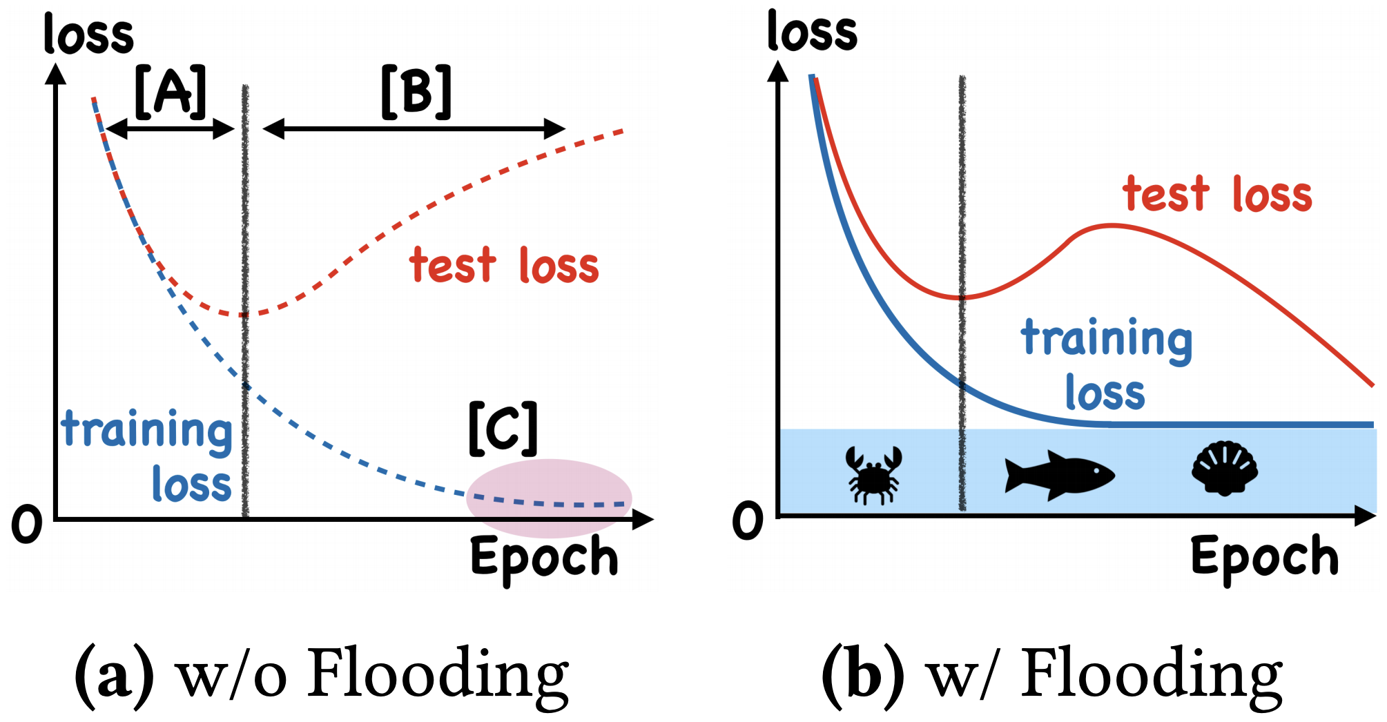Left: training curve without Flooding; right: training curve with Flooding

Put simply, the final validation performance can end up better. The original paper's experimental results are shown below:

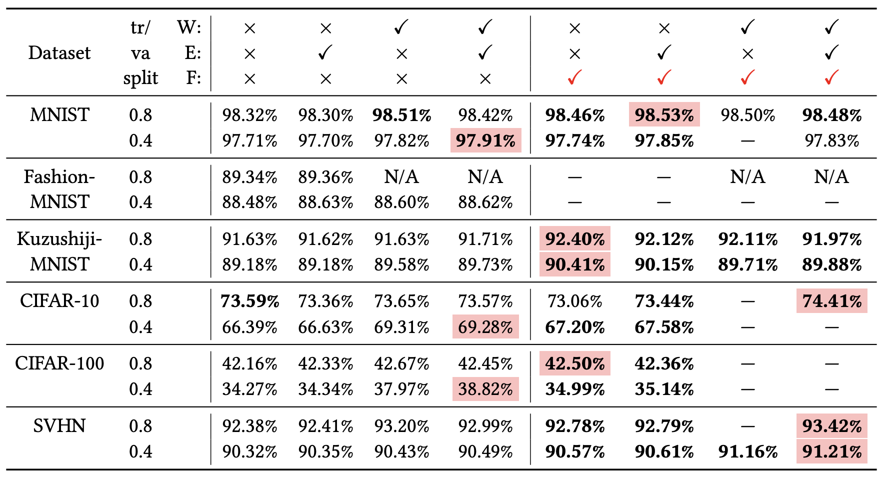Flooding experimental results. Row three, labeled F, denotes Flooding; columns with a red checkmark have Flooding applied.

My own analysis

How can we explain this method? Intuitively, once the loss function reaches $b$, the training process essentially alternates between gradient descent and gradient ascent. Naively, one might think that one ascent step and one descent step should just cancel each other out. Is that really the case? Let's work it out. Suppose we first take a descent step and then an ascent step, with learning rate $\varepsilon$. Then:

\begin{equation}\begin{aligned}&\theta_n = \theta_{n-1} - \varepsilon g(\theta_{n-1})\\ &\theta_{n+1} = \theta_n + \varepsilon g(\theta_n) \end{aligned}\end{equation}

where $g(\theta)=\nabla_{\theta}\mathcal{L}(\theta)$. Now we have

\begin{equation}\begin{aligned}\theta_{n+1} =&\, \theta_{n-1} - \varepsilon g(\theta_{n-1}) + \varepsilon g\big(\theta_{n-1} - \varepsilon g(\theta_{n-1})\big)\\ \approx&\,\theta_{n-1} - \varepsilon g(\theta_{n-1}) + \varepsilon \big(g(\theta_{n-1}) - \varepsilon \nabla_{\theta} g(\theta_{n-1}) g(\theta_{n-1})\big)\\ =&\,\theta_{n-1} - \frac{\varepsilon^2}{2}\nabla_{\theta}\Vert g(\theta_{n-1})\Vert^2 \end{aligned}\end{equation}

Here, $\approx$ is obtained by using a Taylor expansion to approximate the loss function.

The end result is equivalent to gradient descent, with learning rate $\frac{\varepsilon^2}{2}$, on a loss function augmented with the gradient penalty $\Vert g(\theta)\Vert^2=\Vert\nabla_{\theta}\mathcal{L}(\theta)\Vert^2$. Even more elegantly, if we swap the order — "ascent first, then descent" — the resulting expression is exactly the same (this reminds me of the old puzzle about "raising the price by 10% then lowering it by 10%" versus "lowering it by 10% then raising it by 10%"). So, on average, Flooding's modification to the loss function is equivalent to, once the loss is small enough, minimizing $\Vert\nabla_{\theta}\mathcal{L}(\theta)\Vert^2$ as well — that is, pushing the parameters toward flatter regions. This typically improves generalization (better robustness to perturbations), which to some extent explains why Flooding works.

Fundamentally, this isn't really any different from injecting random noise into the parameters, or adversarial training — the only difference here is that the perturbation is only applied after the loss has become sufficiently small. Interested readers can refer to Random Ramblings on Generalization: From Random Noise and Gradient Penalty to Virtual Adversarial Training for related content, or to the "Regularization" section in Part II, Chapter 7 of the "bible" Deep Learning.

Taking the idea further

Readers eager to try this method out might get stuck agonizing over how to choose $b$. But I have another idea: $b$ is really just deciding when to start the alternating training. What if, instead, we alternated between two different learning rates from the very start of training? That is, throughout the entire training process we run

\begin{equation}\begin{aligned}&\theta_n = \theta_{n-1} - \varepsilon_1 g(\theta_{n-1})\\ &\theta_{n+1} = \theta_n + \varepsilon_2 g(\theta_n) \end{aligned}\end{equation}

where $\varepsilon_1 > \varepsilon_2$. This way we eliminate $b$ entirely (though of course we now introduce the choice of $\varepsilon_1/\varepsilon_2$ instead — there's no free lunch). Repeating the same approximation as above, we get

\begin{equation}\begin{aligned} \theta_{n+1} \approx&\, \theta_{n-1} - (\varepsilon_1 - \varepsilon_2) g(\theta_{n-1}) - \frac{\varepsilon_1\varepsilon_2}{2}\nabla_{\theta}\Vert g(\theta_{n-1})\Vert^2\\ =&\,\theta_{n-1} - (\varepsilon_1 - \varepsilon_2)\nabla_{\theta}\left[\mathcal{L}(\theta_{n-1}) + \frac{\varepsilon_1\varepsilon_2}{2(\varepsilon_1 - \varepsilon_2)}\Vert \nabla_{\theta}\mathcal{L}(\theta_{n-1})\Vert^2\right] \end{aligned}\end{equation}

which is equivalent to optimizing the loss function $\mathcal{L}(\theta) + \frac{\varepsilon_1\varepsilon_2}{2(\varepsilon_1 - \varepsilon_2)}\Vert\nabla_{\theta}\mathcal{L}(\theta)\Vert^2$ with learning rate $\varepsilon_1 - \varepsilon_2$ throughout the entire training process — that is, we've baked the gradient penalty in right from the start. Does this actually improve the model's generalization? I tried it out briefly: in some cases there's a slight improvement, and in general it doesn't seem to hurt. But overall it's not as good as directly adding a gradient penalty, so I don't recommend doing it this way.

Note: The reader
@xx205
pointed me to the reference
Backstitch: Counteracting Finite-sample Bias via Negative Steps,
which shows that this approach is effective for speech recognition. So my conclusion above may not be entirely complete — readers should test and judge for themselves. Thanks again to the reader
@xx205
for sharing this material.

Summary

This post gave a brief introduction to the training strategy proposed in an ICML 2020 paper — "switch to gradient ascent once you've gone far enough" — along with my own derivation and interpretation. The result shows that this is equivalent to a gradient penalty on the parameters, and gradient penalty is itself one of the common forms of regularization.