Why Gradient Clipping Accelerates Training: A Concise Analysis

为什么梯度裁剪能加速训练过程？一个简明的分析 苏剑林 · 2020-06-05 · Mathematics optimization gradient

This post introduces a perfect-score ICLR 2020 paper from MIT, Why gradient clipping accelerates training: A theoretical justification for adaptivity. As the title suggests, this paper analyzes why gradient clipping can accelerate the training process of deep learning models. The original paper is long, full of equations, and involves quite a few concepts from complexity theory — honestly, most of it left the author scratching his head — but the core idea can roughly be grasped: it introduces a looser constraint than the commonly used L-constraint, and argues for the necessity of gradient clipping starting from this new condition. This post gives a concise walkthrough of that reasoning, for readers' reference.

Gradient Clipping

Suppose the function we need to minimize is $f(\theta)$, with $\theta$ being the parameters to optimize. Then the gradient descent update rule is

\begin{equation}\theta \leftarrow \theta-\eta \nabla_{\theta} f(\theta)\end{equation}

where $\eta$ is the learning rate. So-called gradient clipping rescales the update based on the norm of the gradient, for example

\begin{equation}\theta \leftarrow \theta- \eta \nabla_{\theta} f(\theta)\times \min\left\{1, \frac{\gamma}{\Vert \nabla_{\theta} f(\theta)\Vert}\right\}\label{eq:clip-1}\end{equation}

or

\begin{equation}\theta \leftarrow \theta- \eta \nabla_{\theta} f(\theta)\times \frac{\gamma}{\Vert \nabla_{\theta} f(\theta)\Vert+\gamma}\label{eq:clip-2}\end{equation}

where $\gamma > 0$ is a constant. Both of these are considered forms of gradient clipping; broadly speaking, both control the norm of the update so that it doesn't exceed a constant, and the second form is also related to adaptive learning-rate optimizers such as RMSProp. Moreover, more precisely, we have the following inequality

\begin{equation}\frac{1}{2}\min\left\{1, \frac{\gamma}{\Vert \nabla_{\theta} f(\theta)\Vert}\right\}\leq \frac{\gamma}{\Vert \nabla_{\theta} f(\theta)\Vert+\gamma}\leq \min\left\{1, \frac{\gamma}{\Vert \nabla_{\theta} f(\theta)\Vert}\right\}\end{equation}

which is to say the two forms bound each other, so they are essentially equivalent. more

The L-Constraint

Many optimizer-related theoretical results assume, in their proofs, that the gradient of the function being optimized $f(\theta)$ satisfies the following L-constraint:

\begin{equation}\Vert \nabla_{\theta} f(\theta + \Delta \theta) - \nabla_{\theta} f(\theta)\Vert\leq L\Vert \Delta\theta\Vert\label{eq:l-cond}\end{equation}

Since $\frac{\Vert \nabla_{\theta} f(\theta + \Delta \theta) - \nabla_{\theta} f(\theta)\Vert}{\Vert \Delta\theta\Vert}$ measures how much the gradient fluctuates, it effectively measures how smooth $f(\theta)$ is, which is why this constraint is also called the "L-smoothness condition" (L-smooth).

The L-constraint has come up several times on this blog before; relevant posts include Lipschitz Constraints in Deep Learning: Generalization and Generative Models] and What Does BN Actually Do? A Closed-Door Analysis]. It's worth noting that different scenarios may call for different L-constraints — sometimes we assume the model's output satisfies an L-constraint with respect to the input, sometimes we assume it does with respect to the parameters, whereas the assumption above is that the gradient of the model's loss satisfies an L-constraint with respect to the parameters.

If condition $\eqref{eq:l-cond}$ holds, many optimization problems become greatly simplified. This is because we can prove (see here] for the derivation) that

\begin{equation}f(\theta+\Delta\theta) \leq f(\theta) + \left\langle \nabla_{\theta}f(\theta), \Delta\theta\right\rangle + \frac{1}{2}L \Vert \Delta\theta\Vert^2\label{eq:neq-1}\end{equation}

For gradient descent, $\Delta\theta = -\eta \nabla_{\theta} f(\theta)$, and substituting this in gives

\begin{equation}f(\theta+\Delta\theta) \leq f(\theta) + \left(\frac{1}{2}L\eta^2 - \eta\right) \Vert \nabla_{\theta}f(\theta)\Vert^2\end{equation}

Therefore, to guarantee that each optimization step causes $f(\theta)$ to decrease, a sufficient condition is $\frac{1}{2}L\eta^2 - \eta < 0$, i.e. $\eta < \frac{2}{L}$. Since $\frac{1}{2}L\eta^2 - \eta$ attains its minimum at $\eta^* = \frac{1}{L} < \frac{2}{L}$, we only need to set the learning rate to $\frac{1}{L}$, and then every iteration will decrease $f(\theta)$, and moreover at the fastest possible rate.

Relaxing the Constraint

The condition $\eqref{eq:l-cond}$ can lead to many elegant results; the problem, however, is that in many real optimization problems condition $\eqref{eq:l-cond}$ simply does not hold — for instance, a quartic function $f(\theta)=\theta^4$ — which creates a gap between theory and practice. The paper introduced here proposes a new, looser constraint:

\begin{equation}\Vert \nabla_{\theta} f(\theta + \Delta \theta) - \nabla_{\theta} f(\theta)\Vert\leq \left(L_0 + L_1\Vert \nabla_{\theta} f(\theta)\Vert\right)\Vert \Delta\theta\Vert\end{equation}

That is, replacing the constant $L$ with the dynamic quantity $L_0 + L_1\Vert \nabla_{\theta} f(\theta)\Vert$. The original paper calls this "(L0, L1)-smooth", which we'll refer to here as the "(L0, L1) constraint." This condition is clearly much more permissive — for example, one can check that $\theta^4$ satisfies it — so theoretical results derived under this condition apply much more broadly.

How did the authors arrive at this condition? According to the paper, it came from experimental observation:

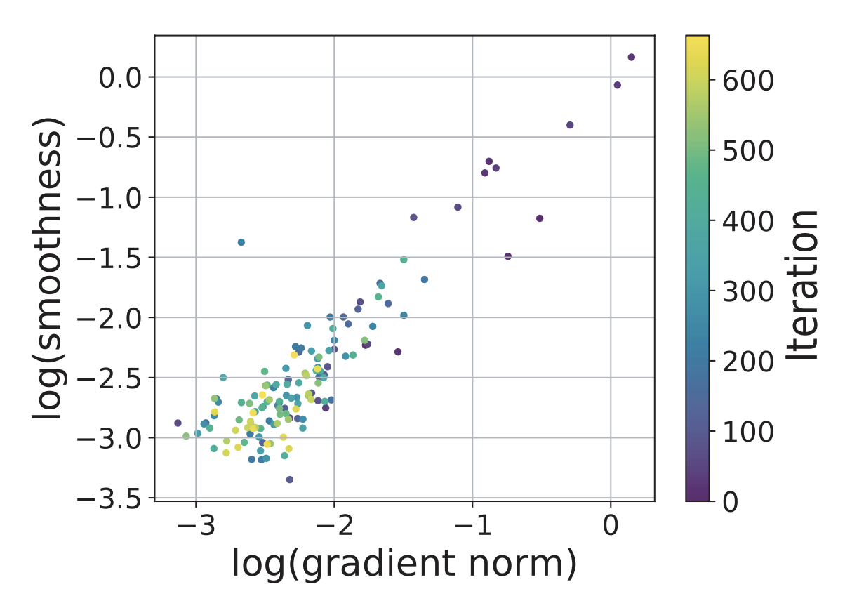The paper observes that the smoothness of the loss function is approximately "linearly correlated" with the gradient norm

That said, the author suspects there's at least some element of reverse-engineering the result here — otherwise, who would be bored enough to go looking for a relationship between these two quantities in the first place?

Under the new constraint, inequality $\eqref{eq:neq-1}$ still holds, except $L$ is replaced by its corresponding dynamic term:

\begin{equation}f(\theta+\Delta\theta) \leq f(\theta) + \left\langle \nabla_{\theta}f(\theta), \Delta\theta\right\rangle + \frac{1}{2}\left(L_0 + L_1\Vert \nabla_{\theta} f(\theta)\Vert\right) \Vert \Delta\theta\Vert^2\end{equation}

Substituting $\Delta\theta = -\eta \nabla_{\theta} f(\theta)$ gives

\begin{equation}f(\theta+\Delta\theta) \leq f(\theta) + \left(\frac{1}{2}\left(L_0 + L_1\Vert \nabla_{\theta} f(\theta)\Vert\right)\eta^2 - \eta\right) \Vert \nabla_{\theta}f(\theta)\Vert^2\end{equation}

So it becomes clear that to guarantee a decrease at every step, we now need

\begin{equation}\eta < \frac{2}{L_0 + L_1\Vert \nabla_{\theta} f(\theta)\Vert}\end{equation}

and the optimal learning rate is

\begin{equation}\eta^* = \frac{1}{L_0 + L_1\Vert \nabla_{\theta} f(\theta)\Vert}\end{equation}

This is exactly what leads to gradient clipping $\eqref{eq:clip-2}$. And guaranteeing a decrease at every step means that no step in the optimization process is wasted — which is precisely why this accelerates training.

Summary

This post gave a brief introduction to a perfect-score ICLR 2020 paper analyzing gradient clipping. The main idea is to introduce a looser, more general assumption, under which the necessity of gradient clipping becomes evident. Because this relaxes the traditional constraint, the resulting theory applies to a much broader range of scenarios — which in turn shows that gradient clipping really is a technique that works well across many settings.