From EMD to WMD to WRD: Computing Similarity Between Text Vector Sequences

从EMD、WMD到WRD：文本向量序列的相似度计算 苏剑林 · 2020-05-13 · Machine Learning optimal optimization semantics linear programming

In NLP, we often need to compare the similarity of two sentences. The standard approach is to encode the sentences into fixed-size vectors, and then use some geometric distance (Euclidean distance, $\cos$ distance, etc.) as the similarity measure. This approach is relatively simple and allows for fast retrieval, which meets engineering needs to a certain extent.

Alternatively, we can directly compare the difference between two variable-length sequences, such as edit distance, which uses dynamic programming to find the optimal mapping between two strings and then computes the degree of mismatch. Nowadays we also have tools like Word2Vec and BERT that can convert a text sequence into a corresponding sequence of vectors, so we can also directly compare these two vector sequences rather than first collapsing each vector sequence into a single vector.

The latter approach is relatively slower, but it allows for finer-grained comparison, and its theoretical foundation is rather elegant, so it also has its own use cases. This post gives a brief introduction to two similarity metrics belonging to this latter category, abbreviated as WMD and WRD.

Earth Mover's Distance

Both metrics introduced in this post are built on the Wasserstein distance, so let's first give a brief introduction to it. Related material can also be found in the author's earlier post From Wasserstein Distance and Duality Theory to WGAN. The Wasserstein distance is also vividly known as the "Earth Mover's Distance" (EMD), because its meaning can be intuitively conveyed through an example about moving earth.more

Optimal transport

Suppose that at location $i=1,2,\dots,n$ we have a pile of earth of amount $p_1,p_2,\dots,p_n$. For simplicity, let's set the total amount of earth to 1, i.e. $p_1 + p_2 + \dots + p_n=1$. Now we want to move this earth to locations $j=1,2,\dots,n'$, where the required amount at each location is $q_1, q_2, \dots, q_{n'}$, and the cost of moving earth from $i$ to $j$ is $d_{i,j}$. We want to find the plan with the lowest cost, and the corresponding minimum cost.

This is precisely a classic optimal transport problem. Let's denote the optimal plan as $\gamma_{i,j}$, meaning that in this plan, an amount $\gamma_{i,j}$ of earth is moved from $i$ to $j$. Clearly we have the constraints

\begin{equation}\sum_j \gamma_{i,j}=p_i,\quad \sum_i \gamma_{i,j}=q_j,\quad \gamma_{i,j} \geq 0\label{eq:cond}\end{equation}

so our optimization problem is

\begin{equation}\min_{\gamma_{i,j} \geq 0} \sum_{i,j} \gamma_{i,j} d_{i,j}\quad \text{s.t.} \quad \sum_j \gamma_{i,j}=p_i,\sum_i \gamma_{i,j}=q_j\end{equation}

Reference implementation

This may look complicated, but on closer inspection you'll notice that the above is just a linear programming problem — finding the extremum of a linear function subject to linear constraints. Since scipy comes with a built-in linear programming solver linprog, we can use it to implement a function for computing the Wasserstein distance:

import numpy as np
from scipy.optimize import linprog

def wasserstein_distance(p, q, D):
    """通过线性规划求Wasserstein距离
    p.shape=[m], q.shape=[n], D.shape=[m, n]
    p.sum()=1, q.sum()=1, p∈[0,1], q∈[0,1]
    """
    A_eq = []
    for i in range(len(p)):
        A = np.zeros_like(D)
        A[i, :] = 1
        A_eq.append(A.reshape(-1))
    for i in range(len(q)):
        A = np.zeros_like(D)
        A[:, i] = 1
        A_eq.append(A.reshape(-1))
    A_eq = np.array(A_eq)
    b_eq = np.concatenate([p, q])
    D = D.reshape(-1)
    result = linprog(D, A_eq=A_eq[:-1], b_eq=b_eq[:-1])
    return result.fun

Readers may notice that when passing in the constraints, we use A_eq=A_eq[:-1], b_eq=b_eq[:-1], i.e., we drop the last constraint. This is because $1=\sum\limits_{i=1}^n p_i = \sum\limits_{j=1}^{n'} q_j$, so the equality constraints in $\eqref{eq:cond}$ are inherently redundant. In practice, floating-point errors can sometimes cause these redundant constraints to contradict each other, causing the linear program to fail to solve. So we simply drop the last redundant constraint to reduce the chance of errors.

Word Mover's Distance

Clearly, the Wasserstein distance is well suited to computing the difference between two sequences of different lengths, and when we're computing semantic similarity, the two sentences in question are typically also of different lengths — which fits this characteristic perfectly. It's therefore natural to wonder whether the Wasserstein distance could be used to compare sentence similarity, and the first attempt at this was made in the paper From Word Embeddings To Document Distances.

Basic form

Suppose we have two sentences $s = (t_1,t_2,\dots,t_n), s' = (t'_1, t'_2, \dots, t'_{n'})$, which, after being passed through some mapping (such as Word2Vec or BERT), become the corresponding vector sequences $(\boldsymbol{w}_1,\boldsymbol{w}_2,\dots,\boldsymbol{w}_n), (\boldsymbol{w}'_1, \boldsymbol{w}'_2, \dots, \boldsymbol{w}'_{n'})$. Now we want to use the Wasserstein distance to compare the similarity of these two sequences.

According to the previous section, the Wasserstein distance requires knowing the three quantities $p_i,q_j,d_{i,j}$, so we just need to define each of them one by one. Since we have no particular prior knowledge, we can simply set $p_i\equiv \frac{1}{n}, q_j\equiv \frac{1}{n'}$, leaving us with $d_{i,j}$. Clearly, $d_{i,j}$ represents some kind of dissimilarity between the vector $\boldsymbol{w}_i$ of the first sequence and the vector $\boldsymbol{w}'_j$ of the second sequence. For simplicity, we can use the Euclidean distance $\left\Vert \boldsymbol{w}_i - \boldsymbol{w}'_j\right\Vert$, so the degree of dissimilarity between the two sentences can be expressed as

\begin{equation}\min_{\gamma_{i,j} \geq 0} \sum_{i,j} \gamma_{i,j} \left\Vert \boldsymbol{w}_i - \boldsymbol{w}'_j\right\Vert\quad \text{s.t.} \quad \sum_j \gamma_{i,j}=\frac{1}{n},\sum_i \gamma_{i,j}=\frac{1}{n'}\end{equation}

This is the Word Mover's Distance (WMD) (the "earth-mover-of-words" distance?). It can roughly be understood as the shortest path for transforming one sentence into another, and in a certain sense can also be understood as a smoothed version of edit distance. In practice, WMD is usually computed after removing stop words.

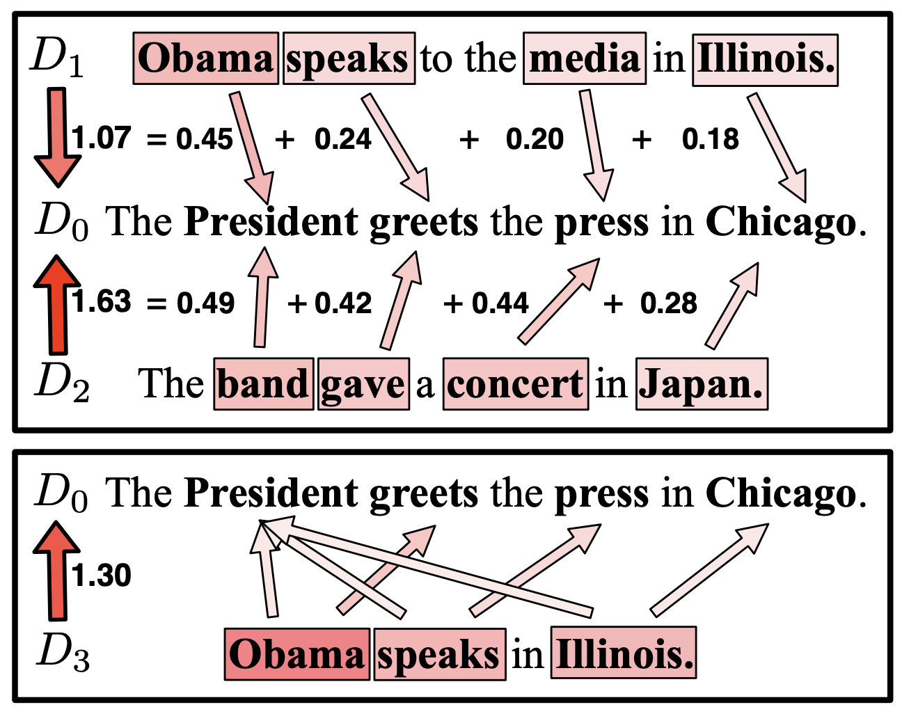Illustration of Word Mover's Distance, from the paper "From Word Embeddings To Document Distances"

Reference implementation

A reference implementation is as follows:

def word_mover_distance(x, y):
    """WMD（Word Mover's Distance）的参考实现
    x.shape=[m,d], y.shape=[n,d]
    """
    p = np.ones(x.shape[0]) / x.shape[0]
    q = np.ones(y.shape[0]) / y.shape[0]
    D = np.sqrt(np.square(x[:, None] - y[None, :]).mean(axis=2))
    return wasserstein_distance(p, q, D)

Lower bound formula

In a retrieval scenario, if we had to compute WMD between an input sentence and every sentence in a database and then sort them, the computational cost would be quite high. So we want to minimize the number of times we compute WMD — for example, by using some cheaper, more efficient metric to filter out some candidates first, and only then computing WMD on the remaining ones.

Fortunately, we can indeed derive a lower bound formula for WMD, which the original paper calls the Word Centroid Distance (WCD):

\begin{equation}\begin{aligned} \sum_{i,j} \gamma_{i,j} \left\Vert \boldsymbol{w}_i - \boldsymbol{w}'_j\right\Vert =& \sum_{i,j} \left\Vert \gamma_{i,j}(\boldsymbol{w}_i - \boldsymbol{w}'_j)\right\Vert\\ \geq& \left\Vert \sum_{i,j}\gamma_{i,j}(\boldsymbol{w}_i - \boldsymbol{w}'_j)\right\Vert\\ =& \left\Vert \sum_i\left(\sum_j\gamma_{i,j}\right)\boldsymbol{w}_i - \sum_j\left(\sum_i\gamma_{i,j}\right)\boldsymbol{w}'_j\right\Vert\\ =& \left\Vert \frac{1}{n}\sum_i\boldsymbol{w}_i - \frac{1}{n'}\sum_j\boldsymbol{w}'_j\right\Vert\\ \end{aligned}\end{equation}

In other words, WMD is greater than the Euclidean distance between the average vectors of the two sentences. So when we want to retrieve sentences with small WMD, we can first use WCD to filter out sentences that are clearly too far away, and only then compute WMD on the remaining candidates.

Word Rotator's Distance

WMD is already quite good, but if we really want to nitpick, we can still find a few shortcomings:

1. It uses Euclidean distance as the measure of semantic difference, but from our experience with Word2Vec, we know that when computing the similarity between word vectors, $\cos$ often works better than Euclidean distance.
2. WMD is, in theory, an unbounded quantity, which means it's hard to intuitively perceive the degree of similarity, and thus difficult to properly set a threshold for "similar vs. not similar."

To address these two issues, a rather naive idea would be to normalize all the vectors by their respective norms before computing WMD, but this would completely discard the norm information. The recent paper Word Rotator's Distance: Decomposing Vectors Gives Better Representations cleverly proposes incorporating the norm into the constraint $p,q$ while still performing the normalization, giving rise to WRD.

Basic form

First, WRD proposes the view that "the norm of a word vector is positively correlated with the importance of that word," and validates this view with some experimental results. In fact, this view is consistent with the view put forward earlier by the author in the simpler glove model; see A More Elegant Word Vector Model (V): Interesting Results. In WMD, $p_i,q_j$ also, in a sense, represents the importance of the corresponding word in the sentence, so we can set

\begin{equation}\begin{aligned}&p_i = \frac{\left\Vert \boldsymbol{w}_i\right\Vert}{Z}, &Z=\sum_{i=1}^n \left\Vert\boldsymbol{w}_i\right\Vert\\ &q_j = \frac{\left\Vert \boldsymbol{w}'_j\right\Vert}{Z'}, &Z'=\sum_{j=1}^{n'}\left\Vert\boldsymbol{w}'_j\right\Vert \end{aligned}\end{equation}

Then for $d_{i,j}$ we use the cosine distance:

\begin{equation}d_{i,j}=1 - \frac{\boldsymbol{w}_i\cdot \boldsymbol{w}'_j}{\left\Vert\boldsymbol{w}_i\right\Vert\times \left\Vert\boldsymbol{w}'_j\right\Vert}\end{equation}

giving us

\begin{equation}\min_{\gamma_{i,j} \geq 0} \sum_{i,j} \gamma_{i,j} \left(1 - \frac{\boldsymbol{w}_i\cdot \boldsymbol{w}'_j}{\left\Vert\boldsymbol{w}_i\right\Vert\times \left\Vert\boldsymbol{w}'_j\right\Vert}\right)\quad \text{s.t.} \quad \sum_j \gamma_{i,j}=\frac{\left\Vert \boldsymbol{w}_i\right\Vert}{Z},\sum_i \gamma_{i,j}=\frac{\left\Vert \boldsymbol{w}'_j\right\Vert}{Z'}\end{equation}

This is the Word Rotator's Distance (WRD). Since it uses cosine distance as the measure, the transformation between the two vectors is more like a rotation than a move — hence the name. Also, because cosine distance is used, its result lies within $[0,2]$, which makes it relatively easier to perceive the degree of similarity.

Reference implementation

A reference implementation is as follows:

def word_rotator_distance(x, y):
    """WRD（Word Rotator's Distance）的参考实现
    x.shape=[m,d], y.shape=[n,d]
    """
    x_norm = (x**2).sum(axis=1, keepdims=True)**0.5
    y_norm = (y**2).sum(axis=1, keepdims=True)**0.5
    p = x_norm[:, 0] / x_norm.sum()
    q = y_norm[:, 0] / y_norm.sum()
    D = 1 - np.dot(x / x_norm, (y / y_norm).T)
    return wasserstein_distance(p, q, D)

def word_rotator_similarity(x, y):
    """1 - WRD
    x.shape=[m,d], y.shape=[n,d]
    """
    return 1 - word_rotator_distance(x, y)

Lower bound formula

Just as with WMD, we can also derive a lower bound formula for WRD:

\begin{equation}\begin{aligned} 2\sum_{i,j} \gamma_{i,j} \left(1 - \frac{\boldsymbol{w}_i\cdot \boldsymbol{w}'_j}{\left\Vert\boldsymbol{w}_i\right\Vert\times \left\Vert\boldsymbol{w}'_j\right\Vert}\right)=&\sum_{i,j} \gamma_{i,j} \left\Vert \frac{\boldsymbol{w}_i}{\left\Vert \boldsymbol{w}_i\right\Vert} - \frac{\boldsymbol{w}'_j}{\left\Vert \boldsymbol{w}'_j\right\Vert}\right\Vert^2 \\ \geq& \left\Vert \sum_{i,j}\gamma_{i,j}\left(\frac{\boldsymbol{w}_i}{\left\Vert \boldsymbol{w}_i\right\Vert} - \frac{\boldsymbol{w}'_j}{\left\Vert \boldsymbol{w}'_j\right\Vert}\right)\right\Vert^2\\ =& \left\Vert \sum_i\left(\sum_j\gamma_{i,j}\right)\frac{\boldsymbol{w}_i}{\left\Vert \boldsymbol{w}_i\right\Vert} - \sum_j\left(\sum_i\gamma_{i,j}\right)\frac{\boldsymbol{w}'_j}{\left\Vert \boldsymbol{w}'_j\right\Vert}\right\Vert^2\\ =& \left\Vert \frac{1}{Z}\sum_i\boldsymbol{w}_i - \frac{1}{Z'}\sum_j\boldsymbol{w}'_j\right\Vert^2\\ \end{aligned}\end{equation}

where the inequality is based on Jensen's inequality (or a generalized version of a basic inequality). This part does not appear in the original WRD paper — it's something the author has added.

Summary, once again

This post has introduced two text similarity algorithms, WMD and WRD, both of which use the Wasserstein distance (Earth Mover's Distance) to directly compare the difference between two variable-length vector sequences. This class of similarity algorithms is somewhat lacking in efficiency, but their theoretical foundation is elegant, and their performance is quite good — well worth learning about.