Variational Autoencoders (V): VAE + BN = A Better VAE

变分自编码器（五）：VAE + BN = 更好的VAE 苏剑林 · 2020-05-06 · Machine Learning variational unsupervised VAE generative model

This post continues our earlier variational autoencoder series, this time analyzing how to prevent the "KL Vanishing" phenomenon that occurs in NLP VAE models. This post was inspired by the ACL 2020 paper A Batch Normalized Inference Network Keeps the KL Vanishing Away, with some further refinements of my own.

It's worth mentioning up front that the solution arrived at here is quite simple — just add BN (Batch Normalization) to the encoder output, then apply a simple scale — but it really works, so it's worth trying for readers currently working on related problems. Moreover, the conclusions here also apply to general VAE models (including those in CV); in my view, it might even be considered "standard equipment" for VAE models.

Finally, a heads-up: this is a fairly advanced VAE post, so it's best read once you already have some background in VAE.

A Quick Review of VAE

Let's briefly review the VAE model and discuss the difficulties VAE runs into in NLP. For a more detailed introduction to VAE, readers can refer to my earlier posts Variational Autoencoders (I): So That's What It Is and Variational Autoencoders (II): From a Bayesian Perspective, among others.

The VAE Training Pipeline

The VAE training pipeline can roughly be illustrated as

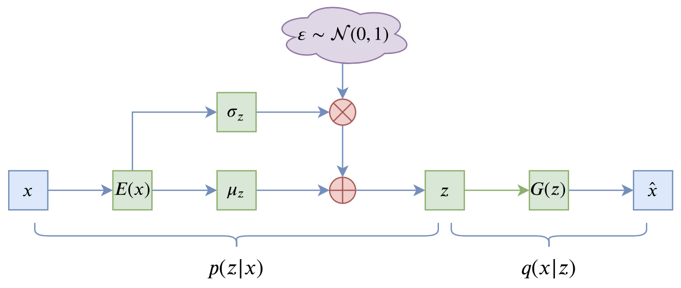Illustration of the VAE training pipelinemore

Written as a formula, this is

$$\begin{equation}\mathcal{L} = \mathbb{E}_{x\sim \tilde{p}(x)} \Big[\mathbb{E}_{z\sim p(z|x)}\big[-\log q(x|z)\big]+KL\big(p(z|x)\big\Vert q(z)\big)\Big] \end{equation}$$

The first term here is the reconstruction term, implemented via $\mathbb{E}_{z\sim p(z|x)}$ through the reparameterization trick; the second term is called the KL divergence term, which is the explicit difference from an ordinary autoencoder — without this term, the model essentially degenerates into a regular AE. For more detail on the notation, see Variational Autoencoders (II): From a Bayesian Perspective.

VAE in NLP

In NLP, sentences are encoded as discrete integer IDs, so $q(x|z)$ is a discrete distribution, which can be implemented using the all-powerful "conditional language model." In theory, then, $q(x|z)$ could fit the generative distribution exactly. The problem is that $q(x|z)$ is too powerful: during training, the reparameterization operation introduces noise, and once the noise gets large, it becomes hard to make use of $z$. So the model simply gives up on $z$ altogether, degenerating into an unconditional language model (still quite powerful), while $KL(p(z|x)\Vert q(z))$ correspondingly collapses to 0 — this is the KL vanishing phenomenon.

A VAE model in this state has essentially no value: a KL divergence of 0 means the encoder is outputting a constant vector, and the decoder is just an ordinary language model. But the whole reason we use VAE is usually its ability to build encoded vectors in an unsupervised way, so if we want to actually apply VAE, we need to solve the KL vanishing problem. In fact, since 2016 there has been a good deal of work on this issue, with many proposed solutions — annealing schedules, alternative priors, and so on. Readers can just Google "KL Vanishing" to find plenty of literature; I won't trace through it all here.

The Cleverness of BN

The approach in this post tackles the KL divergence term directly. It's simple, effective, and involves almost no hyperparameters. The idea is straightforward:

Isn't KL vanishing just the KL term going to 0? What if I adjust the encoder output so that the KL divergence has a lower bound strictly greater than zero? Then it definitely can't vanish.

The direct consequence of this simple idea is: add a BN layer right after $\mu$, as shown below.

Adding BN into a VAE

A Brief Sketch of the Derivation

Why does this connect to BN? Let's look at the form of the KL divergence term:

\begin{equation}\mathbb{E}_{x\sim\tilde{p}(x)}\left[KL\big(p(z|x)\big\Vert q(z)\big)\right] = \frac{1}{b} \sum_{i=1}^b \sum_{j=1}^d \frac{1}{2}\Big(\mu_{i,j}^2 + \sigma_{i,j}^2 - \log \sigma_{i,j}^2 - 1\Big)\end{equation}

The expression above is computed over a sample of $b$ examples, with the encoded vector having dimension $d$. Since we always have $e^x \geq x + 1$, it follows that $\sigma_{i,j}^2 - \log \sigma_{i,j}^2 - 1 \geq 0$, and therefore

\begin{equation}\mathbb{E}_{x\sim\tilde{p}(x)}\left[KL\big(p(z|x)\big\Vert q(z)\big)\right] \geq \frac{1}{b} \sum_{i=1}^b \sum_{j=1}^d \frac{1}{2}\mu_{i,j}^2 = \frac{1}{2}\sum_{j=1}^d \left(\frac{1}{b} \sum_{i=1}^b \mu_{i,j}^2\right)\label{eq:kl}\end{equation}

Notice the quantity inside the parentheses — it's actually just the second moment of $\mu$ within the batch. If we add a BN layer to $\mu$, then we can roughly guarantee that $\mu$ has mean $\beta$ and variance $\gamma^2$ ($\beta,\gamma$ being a trainable parameter within BN), in which case

\begin{equation}\mathbb{E}_{x\sim\tilde{p}(x)}\left[KL\big(p(z|x)\big\Vert q(z)\big)\right] \geq \frac{d}{2}\left(\beta^2 + \gamma^2\right)\label{eq:kl-lb}\end{equation}

So as long as we control $\beta,\gamma$ properly (mainly by fixing $\gamma$ to some constant), we can ensure the KL divergence term has a positive lower bound, which prevents KL vanishing. In this way, the KL vanishing phenomenon becomes neatly connected to BN — BN "rules out" the possibility of KL vanishing.

Why BN and Not LN?

Sharp-eyed readers might notice that, following this same logic, if all we want is a positive lower bound on the KL term, LN (Layer Normalization) should work too — that is, normalizing along the $j$ dimension in equation $\eqref{eq:kl}$.

So why use BN instead of LN?

The answer to this question is itself part of what makes BN clever. Intuitively, KL vanishing happens because the noise in $z\sim p(z|x)$ is relatively large, and the decoder can't reliably distinguish the non-noise component within $z$, so it simply stops using it. When we add BN to $\mu(x)$, this effectively spreads apart the values of $z$ across different samples, so that even with noise added to $z$, distinguishing between samples becomes easier — and the decoder becomes willing to make use of the information in $z$, alleviating the problem. LN, by contrast, normalizes within each individual sample and does nothing to spread samples apart from one another, so LN doesn't work as well as BN.

Further Results

In fact, the derivation in the original paper essentially stops here, with everything else being experimental — including determining the value of $\gamma$ empirically. However, I think the conclusions reached so far leave something to be desired: for one thing, there's no deeper understanding offered of why adding BN works, making it feel more like an engineering trick; for another, only $\mu(x)$ gets BN added while $\sigma(x)$ does not, which feels somewhat asymmetric.

Through my own derivation, I found that the above conclusion can be refined further.

Connecting to the Prior Distribution

For a VAE, the goal is for the trained model's latent variable distribution to match the prior $q(z)=\mathcal{N}(z;0,1)$, while the posterior is $p(z|x)=\mathcal{N}(z; \mu(x),\sigma^2(x))$. So VAE wants the following to hold:

\begin{equation}q(z) = \int \tilde{p}(x)p(z|x)dx=\int \tilde{p}(x)\mathcal{N}(z; \mu(x),\sigma^2(x))dx\end{equation}

Multiplying both sides by $z$ and integrating over $z$, we get

\begin{equation}0 = \int \tilde{p}(x)\mu(x)dx=\mathbb{E}_{x\sim \tilde{p}(x)}[\mu(x)]\end{equation}

Multiplying both sides by $z^2$ and integrating over $z$, we get

\begin{equation}1 = \int \tilde{p}(x)\left[\mu^2(x) + \sigma^2(x)\right]dx = \mathbb{E}_{x\sim \tilde{p}(x)}\left[\mu^2(x)\right] + \mathbb{E}_{x\sim \tilde{p}(x)}\left[\sigma^2(x)\right]\end{equation}

If we add BN to both $\mu(x),\sigma(x)$, then we have

\begin{equation}\begin{aligned} &0 = \mathbb{E}_{x\sim \tilde{p}(x)}[\mu(x)] = \beta_{\mu}\\ &1 = \mathbb{E}_{x\sim \tilde{p}(x)}\left[\mu^2(x)\right] + \mathbb{E}_{x\sim \tilde{p}(x)}\left[\sigma^2(x)\right] = \beta_{\mu}^2 + \gamma_{\mu}^2 + \beta_{\sigma}^2 + \gamma_{\sigma}^2 \end{aligned}\end{equation}

So now we know that $\beta_{\mu}$ must be 0, and if we also fix $\beta_{\sigma}=0$, then we get the constraint relation:

\begin{equation}1 = \gamma_{\mu}^2 + \gamma_{\sigma}^2\label{eq:gamma2}\end{equation}

A Reference Implementation

With this derivation, we see that we can add BN to both $\mu(x),\sigma(x)$ and fix $\beta_{\mu}=\beta_{\sigma}=0$, subject to the constraint $\eqref{eq:gamma2}$. Note that this discussion so far has only been a general analysis of VAE and hasn't yet touched on the KL vanishing problem itself — even if all these conditions are satisfied, there's still no guarantee that the KL term won't tend to 0. Combining this with equation $\eqref{eq:kl-lb}$, we can see that the key to preventing KL vanishing is ensuring $\gamma_{\mu} > 0$. So the final strategy I propose is:

\begin{equation}\begin{aligned} &\beta_{\mu}=\beta_{\sigma}=0\\ &\gamma_{\mu} = \sqrt{\tau + (1-\tau)\cdot\text{sigmoid}(\theta)}\\ &\gamma_{\sigma} = \sqrt{(1-\tau)\cdot\text{sigmoid}(-\theta)} \end{aligned}\end{equation}

where $\tau\in(0,1)$ is a constant — in my own experiments I used $\tau=0.5$ — and $\theta$ is a trainable parameter. The expression above makes use of the identity $\text{sigmoid}(-\theta) = 1-\text{sigmoid}(\theta)$.

Reference implementation (Keras):

class Scaler(Layer):
    """特殊的scale层
    """
    def __init__(self, tau=0.5, **kwargs):
        super(Scaler, self).__init__(**kwargs)
        self.tau = tau

    def build(self, input_shape):
        super(Scaler, self).build(input_shape)
        self.scale = self.add_weight(
            name='scale', shape=(input_shape[-1],), initializer='zeros'
        )

    def call(self, inputs, mode='positive'):
        if mode == 'positive':
            scale = self.tau + (1 - self.tau) * K.sigmoid(self.scale)
        else:
            scale = (1 - self.tau) * K.sigmoid(-self.scale)
        return inputs * K.sqrt(scale)

    def get_config(self):
        config = {'tau': self.tau}
        base_config = super(Scaler, self).get_config()
        return dict(list(base_config.items()) + list(config.items()))

def sampling(inputs):
    """重参数采样
    """
    z_mean, z_std = inputs
    noise = K.random_normal(shape=K.shape(z_mean))
    return z_mean + z_std * noise

e_outputs  # 假设e_outputs是编码器的输出向量
scaler = Scaler()
z_mean = Dense(hidden_dims)(e_outputs)
z_mean = BatchNormalization(scale=False, center=False, epsilon=1e-8)(z_mean)
z_mean = scaler(z_mean, mode='positive')
z_std = Dense(hidden_dims)(e_outputs)
z_std = BatchNormalization(scale=False, center=False, epsilon=1e-8)(z_std)
z_std = scaler(z_std, mode='negative')
z = Lambda(sampling, name='Sampling')([z_mean, z_std])

Summary

This post briefly analyzed the KL vanishing phenomenon that occurs when applying VAE to NLP, and introduced a method for preventing KL vanishing and stabilizing training by adding a BN layer. This is a simple and effective solution — beyond just the original paper, I've also run some informal experiments of my own, and the results do confirm its effectiveness, so it's well worth trying out. Since the derivation is quite general, it's even worth experimenting with in essentially any setting where VAE is used (including CV).