When Bert Meets Keras: Perhaps the Simplest Way to Get Started with Bert

当Bert遇上Keras：这可能是Bert最简单的打开姿势 苏剑林 · 2019-06-18 · Machine Learning language model competition information extraction attention

What Bert is, I probably don't need to introduce at length. Although I'm not particularly fond of Bert, I have to admit it really has stirred up a storm in the NLP world. Whether in Chinese or English, popular explainers and interpretations of Bert are flying all over the place now, arguably even surpassing the momentum Word2Vec had when it first came out. Interestingly, Bert was made by Google, and back then Word2Vec was also made by Google — no matter which one you use, you're always following in Google's footsteps.

Not long after Bert came out, a reader suggested I write an explainer, but in the end I never did. For one thing, there were already plenty of Bert explainers around; for another, Bert is essentially a model built by pretraining on large-scale corpora on top of Attention, which isn't much of a technical innovation in itself, and I had already written an explainer on Google's Attention, so I didn't feel much motivation to write about it.

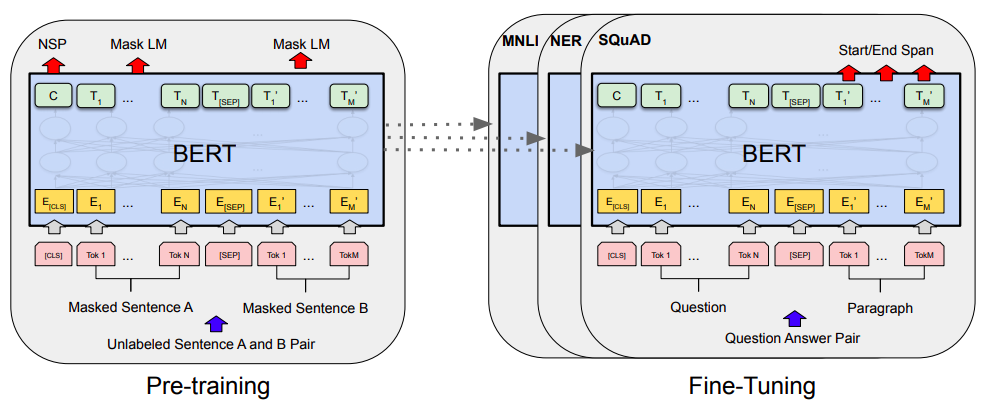Bert pretraining and fine-tuning (image from the original Bert paper)

Overall, I personally never had much interest in Bert, until I first tried it out last month while working on an information extraction competition. Because I eventually figured that even if I'm not interested, I'll eventually need to learn it anyway — whether or not to use it is one thing, but whether you're able to use it is another. Plus, there still didn't seem to be any article introducing how to use (fine-tune) Bert in Keras, so I thought I'd share my experience.more

When Bert Meets Keras

Fortunately, someone has already packaged a Keras version of Bert that lets you directly load the officially released pretrained weights. For readers who already have some Keras background, this may be the simplest way to call Bert. "Standing on the shoulders of giants" describes exactly how we Keras enthusiasts feel right now.

keras-bert

Personally, I think the best Keras wrapper for Bert currently available is:

keras-bert: https://github.com/CyberZHG/keras-bert

This article is also based on it.

By the way, besides keras-bert, the author CyberZHG has also wrapped many other valuable Keras modules, such as keras-gpt-2 (letting you use the GPT-2 model just like Bert), keras-lr-multiplier (setting learning rates by layer), keras-ordered-neurons (which is the ON-LSTM I introduced not long ago), and more — you can find a summary here. Looks like a die-hard Keras fan indeed — hats off.

In fact, with keras-bert plus a bit of basic Keras knowledge, and given that the demos provided with keras-bert are already quite complete, calling and fine-tuning Bert has become something with basically no technical difficulty at all. So below I'll just give a few Chinese-language examples to help readers get familiar with the basic usage of keras-bert.

Tokenizer

Before going into the formal examples, it's worth first discussing the Tokenizer. Let's import Bert's Tokenizer and subclass it a bit:

from keras_bert import load_trained_model_from_checkpoint, Tokenizer
import codecs

config_path = '../bert/chinese_L-12_H-768_A-12/bert_config.json'
checkpoint_path = '../bert/chinese_L-12_H-768_A-12/bert_model.ckpt'
dict_path = '../bert/chinese_L-12_H-768_A-12/vocab.txt'

token_dict = {}
with codecs.open(dict_path, 'r', 'utf8') as reader:
    for line in reader:
        token = line.strip()
        token_dict[token] = len(token_dict)

class OurTokenizer(Tokenizer):
    def _tokenize(self, text):
        R = []
        for c in text:
            if c in self._token_dict:
                R.append(c)
            elif self._is_space(c):
                R.append('[unused1]') # space类用未经训练的[unused1]表示
            else:
                R.append('[UNK]') # 剩余的字符是[UNK]
        return R

tokenizer = OurTokenizer(token_dict)
tokenizer.tokenize(u'今天天气不错')
# 输出是 ['[CLS]', u'今', u'天', u'天', u'气', u'不', u'错', '[SEP]']

Let me briefly explain the output of Tokenizer here. First, by default, [CLS] and [SEP] tags are added at the beginning and end of the sentence after tokenization, where the output vector at the [CLS] position represents a sentence embedding for the whole sentence (that's how Bert is designed anyway), while [SEP] is a separator between sentences, and the rest are per-character outputs (for Chinese).

Originally, Tokenizer has its own _tokenize method, but I've overridden it here to make sure that the tokenized result has the same length as the original string (or, if you count the two tags, the same length plus 2). The built-in _tokenize of Tokenizer automatically strips whitespace, and sometimes certain characters get merged together in the output, which means the tokenized list doesn't match the length of the original string — this can be quite troublesome if you're doing a sequence labeling task. To avoid this trouble, I rewrote it myself: mainly, I use [unused1] to represent whitespace-like characters, and characters not in the vocabulary are represented with [UNK]. The [unused*] tags are untrained (randomly initialized) — they're reserved by Bert for incrementally adding vocabulary, so we can use them to stand in for any new characters.

Three Examples

This covers three examples using keras-bert: text classification, relation extraction, and subject extraction — all fine-tuned on top of the officially released pretrained weights.

Bert's official Github: https://github.com/google-research/bert
Official Chinese pretrained weights: chinese_L-12_H-768_A-12.zip
Github repo for the examples: https://github.com/bojone/bert_in_keras/

According to the official documentation, these weights were trained on the Chinese Wikipedia corpus.

(Update, June 20, 2019: The HIT-iFLYTEK Joint Lab has released a new set of weights, which can also be loaded with keras_bert; see here for details.)

Text Classification

As our first example, let's do the most basic text classification task. Once you're familiar with this basic task, everything else becomes quite simple. This time we'll use the sentiment classification task that we've discussed a number of times before, using the same annotated data compiled previously.

Let's take a look at the full model (see here for the complete code):

# 注意，尽管可以设置seq_len=None，但是仍要保证序列长度不超过512
bert_model = load_trained_model_from_checkpoint(config_path, checkpoint_path, seq_len=None)

for l in bert_model.layers:
    l.trainable = True

x1_in = Input(shape=(None,))
x2_in = Input(shape=(None,))

x = bert_model([x1_in, x2_in])
x = Lambda(lambda x: x[:, 0])(x) # 取出[CLS]对应的向量用来做分类
p = Dense(1, activation='sigmoid')(x)

model = Model([x1_in, x2_in], p)
model.compile(
    loss='binary_crossentropy',
    optimizer=Adam(1e-5), # 用足够小的学习率
    metrics=['accuracy']
)
model.summary()

And that's it — the code for calling Bert to do sentiment classification in Keras is done! Done already!

Feeling like the model code ended too quickly, before you got your fill? That's just how short calling Bert in Keras is. In fact, the only line that actually calls Bert is that single line load_trained_model_from_checkpoint — everything else is ordinary Keras code (thanks again to CyberZHG). So, if you've already gotten a foothold in Keras, calling Bert is smooth sailing.

With such a simple call, what accuracy can you achieve? After 5 epochs of fine-tuning, the best validation accuracy is above 95.5%! Previously, in Text Sentiment Classification (III): To Tokenize or Not to Tokenize, after all sorts of painstaking tuning, we only got around 90% accuracy; but with Bert, in just a handful of lines, accuracy jumped by more than 5 percentage points! No wonder Bert has stirred up such a storm in the NLP world...

Here, let me use my personal experience to answer two questions readers might be curious about.
The first question everyone probably cares about is: "how much GPU memory do I need?" In fact, there's no standard answer — GPU memory usage depends on three factors: sentence length, batch size, and model complexity. Take the sentiment analysis example above: it even runs on my GTX 1060 with 6GB of memory, as long as I set the batch size down to 24. So if your GPU memory isn't big enough, try reducing both maxlen and batch size. Of course, if your task is too complex, no matter how small you make maxlen and batch size, you might still run out of memory — in which case you'll just have to upgrade your graphics card.
The second question is: "what principle should guide what layers to stack on top of Bert?" The answer: use as few layers as possible to accomplish your task. For example, the sentiment analysis above is just a binary classification task — you just take out the first vector and add a Dense(1), no need to stack a bunch more Dense layers, and definitely no need to add an LSTM followed by Dense. If you want to do sequence labeling (like NER), just add a Dense+CRF, and don't add anything else. In short, keep whatever you add on top to a minimum. This is for two reasons: first, Bert itself is already complex enough and has plenty of capacity to handle many tasks; second, whatever layers you add yourself are randomly initialized, and adding too many will severely perturb Bert's pretrained weights, which can easily hurt performance or even cause the model not to converge.

Relation Extraction

Assuming readers already have some Keras background, after going through the first example we should already have a full grasp of fine-tuning Bert, since it's really too simple to need much explanation. So, the next two examples are mainly meant to provide some reference patterns, letting readers experience what "using as few layers as possible to accomplish your task" looks like in practice.

In the second example, we introduce a minimalist relation extraction model built on Bert. The labeling scheme is the same as introduced in A Lightweight Information Extraction Model Based on DGCNN and Probabilistic Graphs, but thanks to Bert's powerful encoding capability, the part we need to write can be greatly simplified. In the reference implementation I give, the model looks like this (see here for the complete model):

t = bert_model([t1, t2])
ps1 = Dense(1, activation='sigmoid')(t)
ps2 = Dense(1, activation='sigmoid')(t)

subject_model = Model([t1_in, t2_in], [ps1, ps2]) # 预测subject的模型

k1v = Lambda(seq_gather)([t, k1])
k2v = Lambda(seq_gather)([t, k2])
kv = Average()([k1v, k2v])
t = Add()([t, kv])
po1 = Dense(num_classes, activation='sigmoid')(t)
po2 = Dense(num_classes, activation='sigmoid')(t)

object_model = Model([t1_in, t2_in, k1_in, k2_in], [po1, po2]) # 输入text和subject，预测object及其关系

train_model = Model([t1_in, t2_in, s1_in, s2_in, k1_in, k2_in, o1_in, o2_in],
                    [ps1, ps2, po1, po2])

If you've already read A Lightweight Information Extraction Model Based on DGCNN and Probabilistic Graphs and understand the model architecture without Bert, you'll appreciate just how concise and clear the above implementation is by comparison.

As you can see, we introduce Bert as the encoder to get the encoded sequence $t$, then directly attach two Dense(1) layers, which completes the subject labeling model. Next, we take the encoded vectors corresponding to the start and end of the given subject s, add them directly onto the encoded vector sequence $t$, and then attach two Dense(num_classes) layers, which completes the object labeling model (simultaneously labeling the relation).

With such a simple design, what F1 score can we end up with? The answer: offline dev gets close to 82%, and on the leaderboard, after one submission, I got 85%+ (both single models)! By comparison, the model in A Lightweight Information Extraction Model Based on DGCNN and Probabilistic Graphs needs a CNN, needs global features, needs to feed s into an LSTM for encoding, and needs relative position vectors — all sorts of hand-tuned modules stitched together — and its single model only performs marginally better (around 82.5%). Keep in mind, this simple Bert-based model took me only an hour to write, while the DGCNN model with all its tricks and combined modules took me nearly two months of debugging on and off! This really shows just how powerful Bert is.

(Note: fine-tuning this model is best done with 8GB or more of GPU memory. Also, because I only got into Bert a few days before the competition ended, and only wrote this Bert-based model at the last minute without spending time carefully tuning it, my final submission didn't actually include Bert.)

One obvious difference between this Bert-based relation extraction example and the earlier simple sentiment analysis example is the learning rate schedule.
In the sentiment analysis example, we just used a constant learning rate ($10^{-5}$) and trained for a few epochs, and the results were already pretty good. In this relation extraction example, the learning rate slowly increases from $0$ to $5\times 10^{-5}$ during the first epoch (this is called warmup), then decreases from $5\times 10^{-5}$ to $10^{-5}$ in the second epoch — overall, it first rises then falls. Bert itself was trained with a similar learning rate curve; this kind of training schedule is more stable, less prone to diverging, and tends to give better results too.

Event Subject Extraction

Our last example comes from CCKS 2019: Event Subject Extraction for the Financial Domain. This competition is still ongoing, but I've already lost the motivation and interest to keep working on it, so I'll release my current model (with accuracy of 89%+) for reference, and wish those still competing the best of luck in achieving even better results.

Briefly, the data for this competition looks something like this:

Input: "Company A's product had an additive issue, and its subsidiaries Company B and Company C were also investigated," "product had a quality issue"
Output: "Company A"

In other words, this is a two-input, single-output model: the input is a query and an event type, and the output is a single entity (exactly one, and it must be a span of the query). This task can actually be viewed as a simplified version of SQUAD 1.0. Given this output characteristic, a pointer structure (two softmaxes predicting the start and end positions separately) works well for the output. The remaining question is: how do we handle the two inputs?

Although the first two examples differ in complexity, they were both single-input. So what do we do with two inputs? Of course, since the number of entity types here is finite, we could just embed them directly — but instead I used an approach that better showcases Bert's brute-force simplicity and power: simply concatenate the two inputs into one sentence using a connector, turning it into a single input! For example, the sample above would be processed into:

Input: "___product had a quality issue___Company A's product had an additive issue, and its subsidiaries Company B and Company C were also investigated"
Output: "Company A"

And then it becomes an ordinary single-input extraction problem. Given this, there's not much to say about the model code either — it's just a few lines (see here for the complete code):

x = bert_model([x1, x2])
ps1 = Dense(1, use_bias=False)(x)
ps1 = Lambda(lambda x: x[0][..., 0] - (1 - x[1][..., 0]) * 1e10)([ps1, x_mask])
ps2 = Dense(1, use_bias=False)(x)
ps2 = Lambda(lambda x: x[0][..., 0] - (1 - x[1][..., 0]) * 1e10)([ps2, x_mask])

model = Model([x1_in, x2_in], [ps1, ps2])

Adding a few decoding tricks plus model ensembling on top of this, and submitting, gets you to 89%+. Looking at the current leaderboard, the best result is just a bit above 90%, so it seems everyone is probably doing roughly the same thing... (This code has fairly high variance when re-run, so try running it a few times and take the best result.)

This example mainly teaches us that when implementing your own task with Bert, it's best to reformulate it as a single-input problem — this is both simpler and more efficient.
For example, when building a sentence-similarity model that takes two sentences as input and outputs a similarity score, there are two approaches that come to mind. The first is to pass each of the two sentences through the same Bert separately and then take their respective [CLS] features for classification. The second, as above, is to join the two sentences into one with a special marker, pass that through a single Bert, and then classify based on the output features. The latter is clearly faster, and also allows for more thorough interaction between the two sets of features.

Summary

This article introduced the basics of calling Bert in Keras, mainly by providing three reference examples to help readers gradually get familiar with the steps and principles behind fine-tuning Bert. Much of this reflects my own experience working things out on my own, so if there are any biases or errors, I welcome readers' corrections.

In fact, with CyberZHG's keras-bert implementation available, using Bert in Keras is a piece of cake — spend half a day tinkering with it, and you'll have it down. Finally, I wish everyone happy hacking~