From the Dynamical Systems Perspective on Optimization Algorithms (IV): The Third Stage of GAN
In the process of learning about and thinking through GANs, I found that I gained not merely an effective generative model, but a deepened understanding of many facets of models in general — the perspective from which to view model optimization, the meaning of regularization terms, the connection between loss functions and probability distributions, probabilistic inference, and so on. GANs are not merely a "toy for forging fakes," but a probabilistic model and inference method of profound significance.
Looking back, I think our understanding of GANs can be roughly divided into three stages:
1. The sample stage: at this stage, we learn the "discriminator-forger" interpretation of GANs, understand how to write down the basic GAN formulas from this principle (e.g., the original GAN, LSGAN) — such as the losses of the discriminator and generator — and manage to train a simple GAN. We also know that GANs have the ability to make images look more "real," and this property can be exploited to embed GANs into various composite models.
2. The distribution stage: at this stage, we analyze GANs from the perspective of probability distributions and their divergences, with WGAN and f-GAN as typical examples. We come to broadly understand the difficulties of GAN training, such as vanishing gradients and mode collapse, and even gain a basic grasp of variational inference, enabling us to write down our own probability divergences and thereby construct new GAN formulations.
3. The dynamical-systems stage: at this stage, we begin to analyze the convergence process of GANs in conjunction with the optimizer, trying to understand whether GANs can actually reach the theoretical equilibrium point, and thereby understand how factors such as the GAN loss and regularization terms affect the convergence process. This allows us to propose targeted training strategies that guide the GAN model toward the theoretical equilibrium point, thereby improving GAN performance.
In fact, this three-stage division applies not just to GANs but, roughly speaking, to the understanding of general models as well. Of course, readers who are fond of geometric or other interpretations might disagree with the second point, feeling that there is no need to insist on understanding things from the angle of probability distributions. But in truth the geometric and probabilistic perspectives share a good deal of common ground, and the three stages described in this post are only a rough summary — in short, the progression is from the local to the global, and then on to the optimizer.
This post focuses mainly on the third stage of GANs: their dynamics.
Basic Principles
In general, a GAN can be expressed as a min-max process, written as
\begin{equation}\min_G \max_D L(G,D)\end{equation}
where step $\max\limits_D L(G,D)$ defines a probability divergence and step $\min\limits_G$ minimizes that divergence. Related discussion can also be found on this site in f-GAN: A Production Line for GAN Models and GANs That Don't Need an L-constraint and Don't Suffer From Vanishing Gradients — Care to Take a Look?.
Note that, in theory, this min-max process is supposed to be ordered: one should complete step $\max\limits_D$ thoroughly and precisely before moving on to $\min\limits_G$. But obviously, when actually training a GAN we cannot do this — we always train $D,G$ alternately, and ideally we would like $D,G$ each to be trained just once per step for maximum training efficiency. Such a training procedure corresponds to a dynamical system.
Dynamical Systems
In our series "From the Dynamical Systems Perspective on Optimization Algorithms," we treat gradient descent as mathematically solving a dynamical system (i.e., a system of ordinary differential equations, ODEs)
\begin{equation}\dot{\boldsymbol{\theta}} = - \nabla_{\boldsymbol{\theta}} L(\boldsymbol{\theta})\end{equation}
where $L(\boldsymbol{\theta})$ is the model's loss and $\boldsymbol{\theta}$ are the model's parameters. If stochasticity is taken into account, one needs to add a noise term, turning this into a stochastic differential equation, but in this post we do not consider stochasticity, since this does not affect our analysis of local convergence. Assuming the reader is already familiar with this conversion, let us go on to discuss the process corresponding to GANs.
A GAN is a min-max process; in other words, one side performs gradient descent while the other performs gradient ascent. Letting $\boldsymbol{\varphi}$ denote the discriminator's parameters and $\boldsymbol{\theta}$ the generator's parameters, the dynamical system corresponding to a GAN is
\begin{equation}\begin{pmatrix}\dot{\boldsymbol{\varphi}}\\ \dot{\boldsymbol{\theta}}\end{pmatrix} = \begin{pmatrix} \nabla_{\boldsymbol{\varphi}} L(\boldsymbol{\varphi},\boldsymbol{\theta})\\ - \nabla_{\boldsymbol{\theta}} L(\boldsymbol{\varphi},\boldsymbol{\theta})\end{pmatrix}\end{equation}
Of course, for more general GANs, the two $L$ terms sometimes differ slightly:
\begin{equation}\begin{pmatrix}\dot{\boldsymbol{\varphi}}\\ \dot{\boldsymbol{\theta}}\end{pmatrix} = \begin{pmatrix} \nabla_{\boldsymbol{\varphi}} L_1(\boldsymbol{\varphi},\boldsymbol{\theta})\\ - \nabla_{\boldsymbol{\theta}} L_2(\boldsymbol{\varphi},\boldsymbol{\theta})\end{pmatrix}\end{equation}
Either way, the two terms on the right-hand side are opposite in sign, and it is precisely this discrepancy between a positive and a negative term that causes the difficulties in GAN training — as we shall gradually come to see below.
Related Work
Treating GAN optimization as a (stochastic) dynamical system is an established viewpoint, and quite a few papers have investigated this. Those I've read include The Numerics of GANs, GANs Trained by a Two Time-Scale Update Rule Converge to a Local Nash Equilibrium, Gradient descent GAN optimization is locally stable, and Which Training Methods for GANs do actually Converge?. This post is nothing more than a study summary of the work of these predecessors.
Of these papers, readers may be most familiar with the second one, since it is the one that proposed the TTUR training strategy for GANs and introduced FID as a performance metric for GANs. That paper's theoretical basis is also to view GAN optimization as the stochastic dynamical system described above, and then to invoke a theorem from stochastic optimization to conclude that the generator and discriminator can be given separate learning rates (TTUR). The remaining papers all directly treat GAN optimization as a deterministic dynamical system (ODEs), and then analyze GANs using the methods of ODE analysis. Since the theoretical analysis and numerical solution of ODEs are both fairly mature fields, many ODE results can be applied directly to GANs.
Dirac GAN
The ideas and results in this post are mainly drawn from Which Training Methods for GANs do actually Converge?, whose main contributions are as follows:
1. It introduces the concept of the Dirac GAN, which allows for a quick, basic grasp of a GAN's behavior;
2. It provides a complete analysis of the local convergence of WGAN with a zero-centered gradient penalty (i.e., WGAN-div);
3. It uses the zero-centered gradient penalty WGAN to generate 1024-resolution faces and 256-resolution LSUN images, without requiring the kind of progressive training used in PGGAN.
Due to hardware limitations, we cannot reproduce point 3, and point 2 involves fairly intricate theoretical analysis that we will not dwell on here — interested readers can go straight to the original paper. This post is mainly concerned with point 1: the Dirac GAN.
The so-called Dirac GAN considers how a given GAN model behaves when the true sample distribution consists of a single point. Suppose the true sample point is the zero vector $\boldsymbol{0}$, and the fake sample is $\boldsymbol{\theta}$, which in fact also represents the generator's parameters; and suppose the discriminator adopts the simplest linear model, i.e., (before the activation function) $D(\boldsymbol{x})=\boldsymbol{x}\cdot \boldsymbol{\varphi}$, where $\boldsymbol{\varphi}$ represents the discriminator's parameters. The Dirac GAN asks whether, under this minimalistic model, the fake sample can ultimately converge to the true sample — that is, whether $\boldsymbol{\theta}$ can eventually converge to $\boldsymbol{0}$.
However, the original paper only considers the case where the sample point is one-dimensional, i.e., $\boldsymbol{0},\boldsymbol{\theta},\boldsymbol{\varphi}$ are all scalars. Later examples in this post will show that, for certain cases, a one-dimensional Dirac GAN is not enough to reveal the true convergence behavior — in general, at least a 2-dimensional Dirac GAN is needed to properly analyze a GAN's asymptotic convergence.
Analysis of Common GANs
In the previous section we introduced the basic concept of the Dirac GAN, and pointed out that it can help us quickly get a sense of a GAN's convergence behavior. In this section, we go through the analysis of several common GANs in more detail to show exactly how the Dirac GAN achieves this.
Vanilla GAN
The Vanilla GAN — also called the original GAN or the standard GAN — refers to the GAN first proposed by Goodfellow, and it comes in two forms: saturating and non-saturating. As an example, let's analyze the more commonly used non-saturating form:
\begin{equation}\begin{aligned}&\min_D \mathbb{E}_{\boldsymbol{x}\sim p(\boldsymbol{x})}[-\log D(\boldsymbol{x})]+\mathbb{E}_{\boldsymbol{x}\sim q(\boldsymbol{x})}[-\log (1-D(\boldsymbol{x}))]\\ &\min_G \mathbb{E}_{\boldsymbol{z}\sim q(\boldsymbol{z})}[-\log D(G(\boldsymbol{z}))] \end{aligned}\end{equation}
Here, $p(\boldsymbol{x}),q(\boldsymbol{x})$ are the true and fake sample distributions respectively, and $q(\boldsymbol{z})$ is the noise distribution, with $D(\boldsymbol{x})$ using a sigmoid activation. Under the Dirac GAN setup this becomes much simpler, since the true distribution is a single point $\boldsymbol{0}$, so the discriminator's loss has only one term, and the discriminator can be written explicitly as $\boldsymbol{\theta}\cdot \boldsymbol{\varphi}$, where $\boldsymbol{\theta}$ is the fake sample, i.e., the generator. The final result is:
\begin{equation}\begin{aligned}&\min_{\boldsymbol{\varphi}} -\log (1-\sigma(\boldsymbol{\theta}\cdot \boldsymbol{\varphi}))\\ &\min_{\boldsymbol{\theta}} -\log \sigma(\boldsymbol{\theta}\cdot \boldsymbol{\varphi}) \end{aligned}\end{equation}
The corresponding dynamical system is:
\begin{equation}\begin{pmatrix}\dot{\boldsymbol{\varphi}}\\ \dot{\boldsymbol{\theta}}\end{pmatrix} = \begin{pmatrix} \nabla_{\boldsymbol{\varphi}} \log (1-\sigma(\boldsymbol{\theta}\cdot \boldsymbol{\varphi}))\\ \nabla_{\boldsymbol{\theta}} \log \sigma(\boldsymbol{\theta}\cdot \boldsymbol{\varphi})\end{pmatrix} = \begin{pmatrix} - \sigma(\boldsymbol{\theta}\cdot \boldsymbol{\varphi}) \boldsymbol{\theta}\\ (1 - \sigma(\boldsymbol{\theta}\cdot \boldsymbol{\varphi}))\boldsymbol{\varphi}\end{pmatrix}\end{equation}
The equilibrium point of this dynamical system (setting the right-hand side to zero) is $\boldsymbol{\varphi}=\boldsymbol{\theta}=\boldsymbol{0}$, i.e., the fake sample becomes the true sample. But the question is whether, starting from an arbitrary initial point, that initial point will actually converge to this equilibrium — this is not obvious at all.
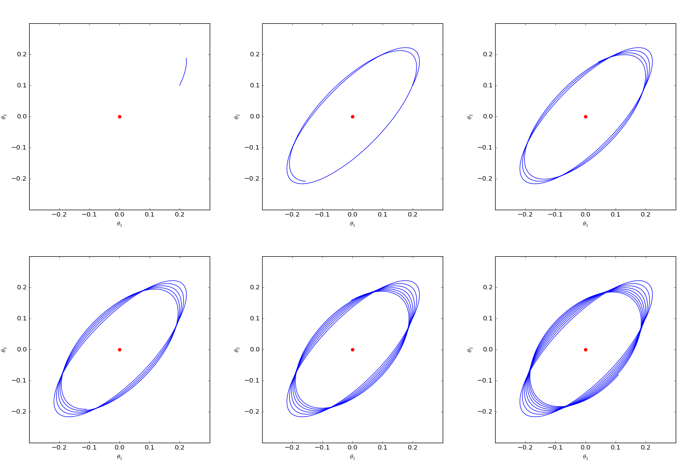 Numerically solved optimization trajectory of the non-saturating Dirac GAN (2D case); one observes that it only oscillates around the equilibrium point (red dot) rather than converging
To make this judgment, suppose the system has already run to near the equilibrium point, i.e., $\boldsymbol{\varphi}\approx \boldsymbol{0}, \boldsymbol{\theta}\approx \boldsymbol{0}$, so that we can approximately linearize:
\begin{equation}\begin{pmatrix}\dot{\boldsymbol{\varphi}}\\ \dot{\boldsymbol{\theta}}\end{pmatrix} = \begin{pmatrix} - \sigma(\boldsymbol{\theta}\cdot \boldsymbol{\varphi}) \boldsymbol{\theta}\\ (1 - \sigma(\boldsymbol{\theta}\cdot \boldsymbol{\varphi}))\boldsymbol{\varphi}\end{pmatrix} \approx \begin{pmatrix} - \boldsymbol{\theta} / 2\\ \boldsymbol{\varphi} / 2\end{pmatrix}\end{equation}
which finally gives, approximately,
\begin{equation}\ddot{\boldsymbol{\theta}}\approx - \boldsymbol{\theta} / 4\end{equation}
Anyone who has studied ordinary differential equations will recognize this as one of the simplest possible linear ODEs: as long as the initial value is not $\boldsymbol{0}$, the solution is periodic — that is, there is no $\boldsymbol{\theta}\to \boldsymbol{0}$ behavior. In other words, for the non-saturating Vanilla GAN, even if the model's initialization is already quite close to the equilibrium, it will never converge to the equilibrium point, but will instead oscillate around it forever. Numerical simulation further confirms this.
In fact, similar results occur for any form of f-GAN — that is, all GANs based on an f-divergence suffer from the same problem (ignoring regularization terms): they slowly approach the neighborhood of the equilibrium point, but ultimately just oscillate around it, never fully converging to it.
Let us restate the logic here: we know the theoretical equilibrium point of the system is indeed what we want, but starting from an arbitrary initial value (corresponding to the model's initialization), whether iteration will eventually reach the theoretical equilibrium (corresponding to ideally completing GAN training) is not obvious — at the very least, one needs to linearize near the equilibrium point and analyze its convergence behavior. This is what is meant by so-called local asymptotic convergence behavior.
WGAN
So f-GAN has fallen down on this front — what about WGAN? Can it converge to the desired equilibrium?
The general form of WGAN is
\begin{equation}\min_G \max_{D, \Vert D\Vert_L\leq 1} \mathbb{E}_{\boldsymbol{x}\sim p(\boldsymbol{x})}[D(\boldsymbol{x})] - \mathbb{E}_{\boldsymbol{z}\sim q(\boldsymbol{z})}[D(G(\boldsymbol{z}))]\end{equation}
Under the Dirac GAN setup, $D(\boldsymbol{x})=\boldsymbol{x}\cdot \boldsymbol{\varphi}$, and $\Vert D\Vert_L\leq 1$ can be enforced by $\Vert \boldsymbol{\varphi}\Vert=1$ ($\Vert\cdot\Vert$ being the norm of $l_2$). In other words, $D(\boldsymbol{x})$ subject to the L-constraint becomes $D(\boldsymbol{x})=\boldsymbol{x}\cdot \boldsymbol{\varphi} / \Vert\boldsymbol{\varphi}\Vert$, so that the WGAN's corresponding Dirac GAN is
\begin{equation}\min_{\boldsymbol{\theta}}\max_{\boldsymbol{\varphi}} \frac{-\boldsymbol{\theta}\cdot \boldsymbol{\varphi}}{\Vert\boldsymbol{\varphi}\Vert}\end{equation}
with corresponding dynamical system:
\begin{equation}\begin{pmatrix}\dot{\boldsymbol{\varphi}}\\ \dot{\boldsymbol{\theta}}\end{pmatrix} = \begin{pmatrix} \nabla_{\boldsymbol{\varphi}} (-\boldsymbol{\theta}\cdot \boldsymbol{\varphi} / \Vert \boldsymbol{\varphi}\Vert)\\ \nabla_{\boldsymbol{\theta}} (\boldsymbol{\theta}\cdot \boldsymbol{\varphi} / \Vert \boldsymbol{\varphi}\Vert)\end{pmatrix} = \begin{pmatrix} -\boldsymbol{\theta} / \Vert \boldsymbol{\varphi}\Vert + (\boldsymbol{\theta}\cdot \boldsymbol{\varphi})\boldsymbol{\varphi} / \Vert \boldsymbol{\varphi}\Vert^3\\ \boldsymbol{\varphi} / \Vert \boldsymbol{\varphi}\Vert\end{pmatrix}\end{equation}
We are mainly interested in whether $\boldsymbol{\theta}$ tends toward $\boldsymbol{0}$. We could introduce a linear expansion similar to the previous section, but since $\Vert \boldsymbol{\varphi}\Vert$ appears in the denominator, this makes the discussion rather cumbersome. The most straightforward approach is to directly numerically solve this system of equations, with the results shown below:
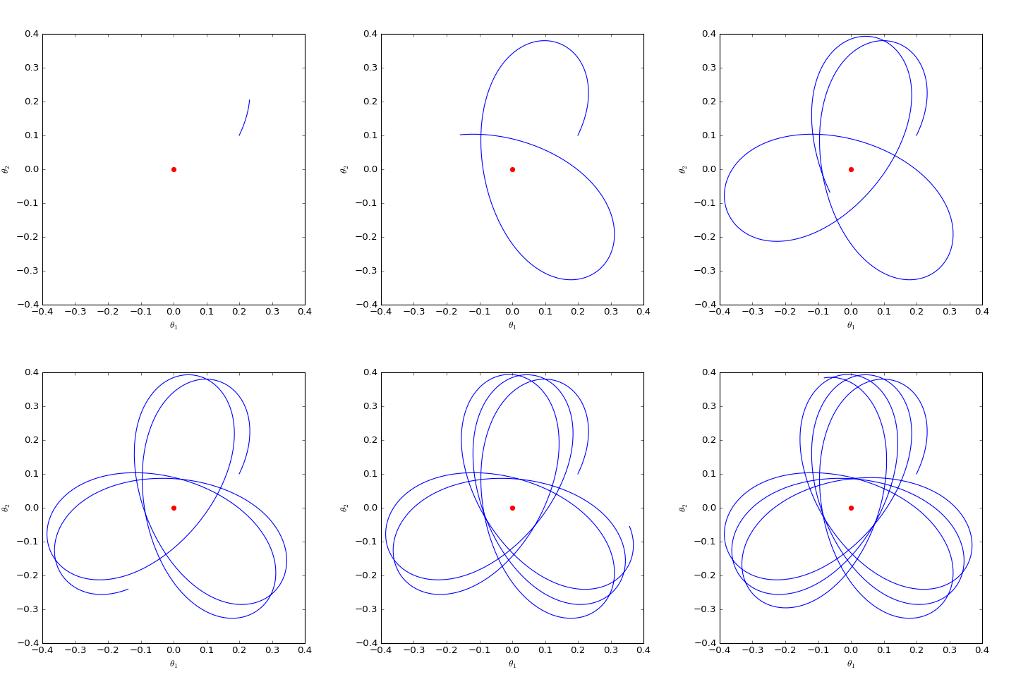 Numerically solved optimization trajectory of the Dirac GAN corresponding to WGAN (2D case); one observes that it also only oscillates around the equilibrium point (red dot) rather than converging
As we can see, the result again oscillates around the equilibrium point without ever reaching it. This tells us that WGAN (and naturally also spectral normalization) does not have local convergence — even after having reached the neighborhood of the equilibrium, it still cannot land precisely on it.
(Note: a little analysis shows that if we only consider the one-dimensional Dirac GAN, we would be unable to analyze the WGAN discussed here or the GAN-QP discussed later — this is exactly the limitation of restricting to the one-dimensional case.)
WGAN-GP
Some readers might be puzzled: didn't we already discuss WGAN above — why discuss WGAN-GP as well?
In fact, from an optimization standpoint, the WGAN discussed earlier and WGAN-GP are two different types of models. The WGAN above refers to imposing the L-constraint on the discriminator in advance (e.g. via spectral normalization) before performing adversarial training; WGAN-GP here refers to a discriminator without an explicit L-constraint, which is instead enforced via a Gradient Penalty term. There are two forms of gradient penalty discussed here: the first is the "1-centered gradient penalty" proposed in Improved Training of Wasserstein GANs, and the second is the "0-centered gradient penalty" advocated by papers such as Wasserstein Divergence for GANs and Which Training Methods for GANs do actually Converge?. Below we compare the different behaviors of these two gradient penalties.
The general form of the gradient penalty is:
\begin{equation}\begin{aligned}&\min_{D} \mathbb{E}_{\boldsymbol{x}\sim q(\boldsymbol{x})}[D(\boldsymbol{x})] - \mathbb{E}_{\boldsymbol{x}\sim p(\boldsymbol{x})}[D(\boldsymbol{x})] + \lambda \mathbb{E}_{\boldsymbol{x}\sim r(\boldsymbol{x})}\left[(\left\Vert\nabla_{\boldsymbol{x}}D(\boldsymbol{x})\right\Vert - c)^2\right]\\ &\min_{G} \mathbb{E}_{\boldsymbol{z}\sim q(\boldsymbol{z})}[-D(G(\boldsymbol{z}))] \end{aligned}\end{equation}
where $c=0$ or $c=1$, and $r(\boldsymbol{x})$ is some derived distribution from $p(\boldsymbol{x})$ and $q(\boldsymbol{x})$ — typically taken directly to be the true distribution, the fake distribution, or an interpolation between real and fake samples.
For the Dirac GAN:
\begin{equation}\nabla_{\boldsymbol{x}}D(\boldsymbol{x}) = \nabla_{\boldsymbol{x}}(\boldsymbol{x}\cdot\boldsymbol{\varphi})=\boldsymbol{\varphi}\end{equation}
which is to say that this term has nothing to do with $\boldsymbol{x}$, so however $r(\boldsymbol{x})$ is chosen makes no difference to the result. Hence, the WGAN-GP version of the Dirac GAN takes the form:
\begin{equation}\begin{aligned}&\min_{\boldsymbol{\varphi}} \boldsymbol{\theta}\cdot\boldsymbol{\varphi} + \lambda (\left\Vert \boldsymbol{\varphi}\right\Vert - c)^2\\ &\min_{\boldsymbol{\theta}} -\boldsymbol{\theta}\cdot\boldsymbol{\varphi}\end{aligned}\end{equation}
with corresponding dynamical system:
\begin{equation}\begin{pmatrix}\dot{\boldsymbol{\varphi}}\\ \dot{\boldsymbol{\theta}}\end{pmatrix} = \begin{pmatrix} \nabla_{\boldsymbol{\varphi}} (-\boldsymbol{\theta}\cdot\boldsymbol{\varphi} - \lambda (\left\Vert \boldsymbol{\varphi}\right\Vert - c)^2)\\ \nabla_{\boldsymbol{\theta}} (\boldsymbol{\theta}\cdot\boldsymbol{\varphi})\end{pmatrix} = \begin{pmatrix} -\boldsymbol{\theta} - 2\lambda (1 - c / \Vert \boldsymbol{\varphi}\Vert) \boldsymbol{\varphi} \\ \boldsymbol{\varphi} \end{pmatrix}\end{equation}
Let's examine, for the two cases of $c=0,c=1$, whether $\boldsymbol{\theta}$ tends toward $\boldsymbol{0}$. When $c=0$, this is actually just a linear system of ODEs and can be solved analytically, but when $c=1$ it becomes more complicated, so for simplicity we again solve it numerically:
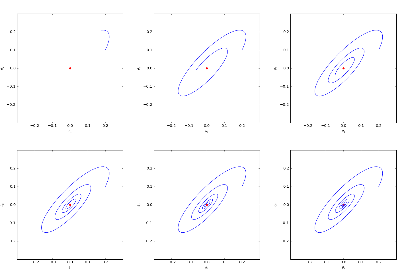 Numerically solved optimization trajectory of the Dirac GAN corresponding to WGAN-GP (c=0) (2D case); one observes that it can converge asymptotically to the equilibrium point (red dot)
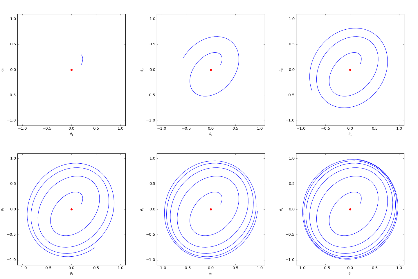 Numerically solved optimization trajectory of the Dirac GAN corresponding to WGAN-GP (c=1) (2D case); one observes that it only oscillates around the equilibrium point (red dot) rather than converging
The figures above show, under identical initial conditions, the different behaviors resulting from the two choices of $c=0,c=1$ gradient penalty, with all other parameters kept the same. We can see that with the "1-centered gradient penalty," the Dirac GAN does not converge asymptotically to the origin, but instead only converges onto a circle; whereas the "0-centered gradient penalty" successfully achieves convergence to the equilibrium. This shows that the earlier-proposed gradient penalty term does indeed have certain defects, and the "0-centered gradient penalty" is better behaved in terms of convergence. Although we've only performed this analysis on the Dirac GAN, the conclusion is representative, since a general proof of the superiority of the zero-centered gradient penalty is already given in Which Training Methods for GANs do actually Converge?, and confirmed by experiments.
GAN-QP
Finally, let's look at how the GAN-QP I proposed myself performs. Compared to WGAN-GP, GAN-QP replaces the gradient penalty with a quadratic difference penalty term, along with some supplementary proofs. Compared to the gradient penalty, the main advantage of the difference penalty is faster computation.
GAN-QP can take various forms; one basic form is:
\begin{equation}\begin{aligned}&\min_{D} \mathbb{E}_{\boldsymbol{x}_r\sim p(\boldsymbol{x}_r),\boldsymbol{x}_f\sim q(\boldsymbol{x}_f)}\left[D(\boldsymbol{x}_f) - D(\boldsymbol{x}_r) + \frac{(D(\boldsymbol{x}_f) - D(\boldsymbol{x}_r))^2}{2\lambda \Vert \boldsymbol{x}_f - \boldsymbol{x}_r\Vert}\right]\\ &\min_{G} \mathbb{E}_{\boldsymbol{z}\sim q(\boldsymbol{z})}[-D(G(\boldsymbol{z}))] \end{aligned}\end{equation}
whose corresponding Dirac GAN is
\begin{equation}\begin{aligned}&\min_{\boldsymbol{\varphi}} \boldsymbol{\theta}\cdot\boldsymbol{\varphi} + \frac{(\boldsymbol{\theta}\cdot\boldsymbol{\varphi})^2}{2\lambda \Vert \boldsymbol{\theta}\Vert}\\ &\min_{\boldsymbol{\theta}} -\boldsymbol{\theta}\cdot\boldsymbol{\varphi}\end{aligned}\end{equation}
with corresponding dynamical system:
\begin{equation}\begin{pmatrix}\dot{\boldsymbol{\varphi}}\\ \dot{\boldsymbol{\theta}}\end{pmatrix} = \begin{pmatrix} \nabla_{\boldsymbol{\varphi}} (-\boldsymbol{\theta}\cdot\boldsymbol{\varphi} - (\boldsymbol{\theta}\cdot\boldsymbol{\varphi})^2 / (2\lambda \Vert \boldsymbol{\theta}\Vert))\\ \nabla_{\boldsymbol{\theta}} (\boldsymbol{\theta}\cdot\boldsymbol{\varphi})\end{pmatrix} = \begin{pmatrix} -\boldsymbol{\theta} - (\boldsymbol{\theta}\cdot\boldsymbol{\varphi})\boldsymbol{\theta}/(\lambda \Vert \boldsymbol{\theta}\Vert)\\ \boldsymbol{\varphi} \end{pmatrix}\end{equation}
The numerical results are shown below (first figure):
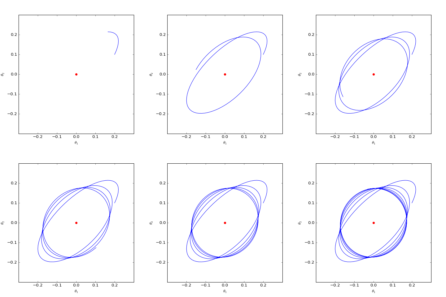 Numerically solved optimization trajectory of the Dirac GAN corresponding to GAN-QP (2D case); one observes that it also only oscillates around the equilibrium point (red dot) rather than converging
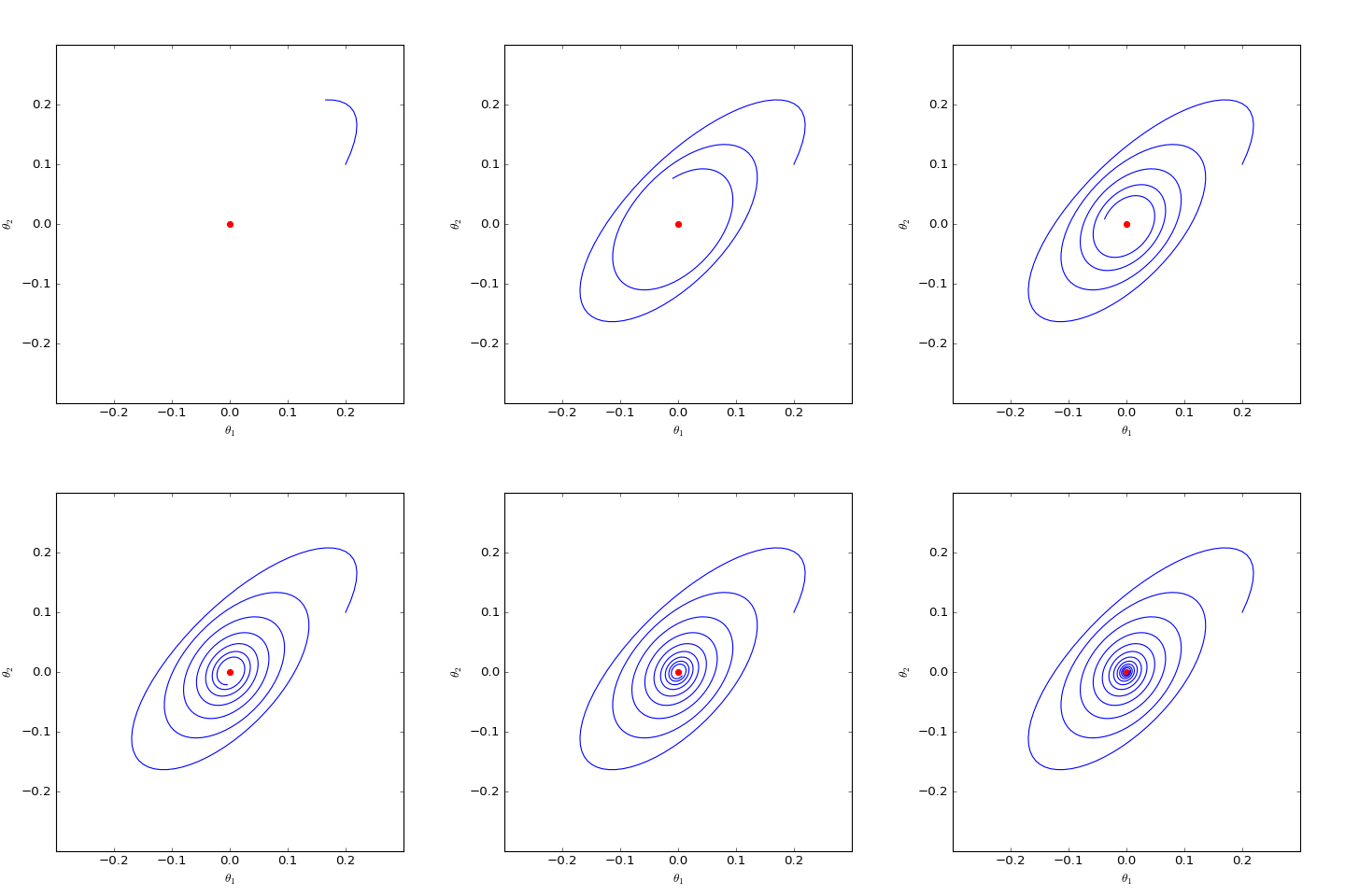 Numerically solved GAN-QP Dirac GAN version with an L2 regularization term added, all other conditions kept the same as before — this suggests that a suitable L2 regularization term may induce convergence
Unfortunately, like most GANs, GAN-QP also oscillates.
Mitigation Strategies
From the analysis above, we conclude that, at present, the zero-centered WGAN-GP (also known as WGAN-div) has the best theoretical properties — it is the only one that is locally convergent, while all the other GAN variants exhibit some degree of oscillation and cannot truly achieve asymptotic convergence. Of course, real-world situations may be far more complicated, and the conclusions from Dirac GAN can only illustrate the issue to a certain degree, offering an intuitive sense of the phenomenon.
So, if the conclusions from Dirac GAN are indeed representative (i.e., in practice most GANs struggle to truly converge, oscillating around the equilibrium point instead), how should we go about mitigating this problem?
L2 Regularization
The first approach is to consider adding an L2 regularization term to the weights of the discriminator (for any GAN). As discussed above, the zero-centered gradient penalty does perform very well, but unfortunately the gradient penalty is computationally expensive. If one prefers not to add a gradient penalty, adding an L2 regularization term is an alternative worth considering.
Intuitively, a GAN gets trapped in oscillation near the equilibrium point, reaching a kind of dynamic equilibrium (a periodic solution rather than a static one), and the L2 regularization term pulls the discriminator's weights toward zero, which can potentially break this equilibrium — as shown in the second figure above. In my own GAN experiments, adding a mild L2 regularization term to the discriminator makes the model converge more stably and slightly improves the results. (Of course, the weight of the regularization term needs to be tuned to fit the model.)
Exponential Moving Average of Weights
In fact, the most powerful technique for mitigating this problem is undoubtedly exponential moving average (EMA) of the weights.
The basic idea of the EMA of weights was already introduced in "Making Keras Even Cooler!": Intermediate Variables, Weight Averaging, and Safe Generators. Applying it to GANs isn't hard to understand, because we can observe that although most GANs end up oscillating, the center of oscillation is precisely the equilibrium point! So the solution is simple: just average the points along the oscillating trajectory to get an approximation of this center, and thereby obtain a solution closer to the equilibrium (i.e., higher quality)!
The improvement brought about by weight moving averages is quite substantial, as shown in the figure below, comparing O-GAN's generative outputs with and without the EMA of weights:
 Random generation results without EMA of weights
 Random generation results with EMA of weights, decay rate 0.999
 Random generation results with EMA of weights, decay rate 0.9999
As we can see, the EMA of weights brings an almost qualitative improvement to the generation quality. The larger the decay rate, the smoother the generated results, but at the cost of losing some detail; the smaller the decay rate, the more detail is retained, but it may also retain extra noise. Nowadays mainstream GANs generally use EMA of weights, typically with a decay rate around 0.999.
Incidentally, in ordinary supervised training as well, EMA of weights generally speeds up convergence. For example, the figure below shows the training curves of a ResNet20 model on CIFAR-10 with and without EMA of weights, trained throughout with the Adam optimizer at a constant learning rate of 0.001, with an EMA decay rate of 0.9999:
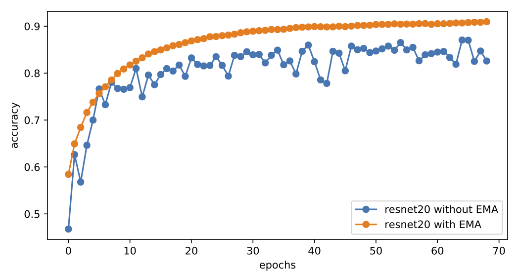 Performance of training ResNet20 with Adam at its default learning rate, with and without EMA
We can see that, with the EMA of weights added, the model converges to an accuracy of 90%+ in a very smooth and rapid manner, whereas without it, model accuracy keeps oscillating around 86%. This shows that oscillation phenomena similar to those seen in GANs are common in deep learning training in general, and averaging the weights can yield a higher-quality model.
Summary
This post has explored the optimization problem of GANs from a dynamical-systems perspective. As with other posts in this series, we treat the optimization process as the solution of a system of ordinary differential equations — for GAN optimization, this system of ODEs is a bit more complicated.
The analysis proceeds using the Dirac GAN approach, using the minimalist scenario of a single-point distribution to quickly develop intuition about the convergence process of GANs. The conclusion is that most GANs cannot truly converge to the equilibrium point, but instead only oscillate around it. To mitigate this problem, the most powerful method is the EMA of weights, which is helpful both for GAN training and for ordinary model training in general.
(Code for the figures in this post can be found at: https://github.com/bojone/gan/blob/master/gan_numeric.py)
Translated automatically with claude-sonnet-5; all equations are reproduced verbatim from the source. Copyright remains with the original author.