Viewing Optimizers from the Perspective of Dynamics (I): From SGD to Momentum Acceleration
In this series, we're going to focus on optimization algorithms, and the theme of this article is SGD (stochastic gradient descent), including the Momentum and Nesterov variants. For SGD, the questions we usually care about include:
Why does SGD work?
Is a bigger batch size always better for SGD?
How should the learning rate be tuned in SGD?
How does Momentum achieve acceleration?
Why is Nesterov slightly better than Momentum?
...
Here we try to analyze SGD from the perspective of dynamics, offering some suggestive understanding of the questions above.
Gradient Descent
Since we want to compare which method is better or worse, we first need to know what "best" looks like — that is, what is our ultimate goal?
Analyzing the training objective
Suppose the full set of training samples is $\boldsymbol{S}$, and the loss metric is $L(\boldsymbol{x};\boldsymbol{\theta})$, where $\boldsymbol{x}$ represents a single sample and $\boldsymbol{\theta}$ is the parameter to be optimized. Then we can construct the loss function
$$L(\boldsymbol{\theta}) = \frac{1}{|\boldsymbol{S}|}\sum_{\boldsymbol{x}\in\boldsymbol{S}} L(\boldsymbol{x};\boldsymbol{\theta})\tag{1}$$
and the ultimate goal of training is to find a global optimum of $L(\boldsymbol{\theta})$ (here "optimum" means "minimum"). more
GD and ODEs
To achieve this goal, we can use gradient descent (GD):
$$\boldsymbol{\theta}_{n+1}=\boldsymbol{\theta}_{n} - \gamma \nabla_{\boldsymbol{\theta}} L(\boldsymbol{\theta}_{n})\tag{2}$$
where $\gamma > 0$ is called the learning rate, which here also happens to be the step size of the iteration (later we'll see that the step size need not equal the learning rate). There are many ways to understand gradient descent; since generally $\gamma \ll 1$ holds, we can rewrite this as
$$\frac{\boldsymbol{\theta}_{n+1}-\boldsymbol{\theta}_{n}}{\gamma} = - \nabla_{\boldsymbol{\theta}} L(\boldsymbol{\theta}_{n})\tag{3}$$
Then the left-hand side approximates the derivative of $\boldsymbol{\theta}$ (assuming it is a function of time $t$), so we obtain the ODE dynamical system:
$$\dot{\boldsymbol{\theta}} = - \nabla_{\boldsymbol{\theta}} L(\boldsymbol{\theta})\tag{4}$$
and $(2)$ is an Euler solution of $(4)$. In other words, gradient descent is essentially using the Euler method to solve the dynamical system $(4)$. Since $(4)$ is a conservative dynamical system, it will eventually converge to a fixed point (where $\dot{\boldsymbol{\theta}}=0$), and it can be shown that a stable fixed point is a local minimum (though not necessarily the global minimum).
Stochastic Gradient Descent
Here we show that stochastic gradient descent can be analyzed, semi-qualitatively and semi-quantitatively, using a stochastic differential equation.
From GD to SGD
$(2)$ is generally called "full-batch gradient descent," because it requires all the samples to compute the gradient — this is a notable drawback of gradient descent: when there are tens of thousands of samples, the cost of each iteration becomes too large, potentially even infeasible. So instead we want to randomly draw a subset $\boldsymbol{R}\subseteq \boldsymbol{S}$ from $\boldsymbol{S}$, and use only $\boldsymbol{R}$ to compute the gradient and complete a single iteration. We denote
$$L_{\boldsymbol{R}}(\boldsymbol{\theta}) = \frac{1}{|\boldsymbol{R}|}\sum_{\boldsymbol{x}\in\boldsymbol{R}} L(\boldsymbol{x};\boldsymbol{\theta})\tag{5}$$
Then formula $(2)$ becomes
$$\boldsymbol{\theta}_{n+1}=\boldsymbol{\theta}_{n} - \gamma \nabla_{\boldsymbol{\theta}} L_{\boldsymbol{R}}(\boldsymbol{\theta}_{n})\tag{6}$$
Note that it's the minimum of $L$ that is our actual goal, while $L_{\boldsymbol{R}}$ is a random variable — $\nabla_{\boldsymbol{\theta}} L_{\boldsymbol{R}}(\boldsymbol{\theta}_{n})$ is merely an estimate of the original $\nabla_{\boldsymbol{\theta}} L(\boldsymbol{\theta}_{n})$. Can this approach still yield a reasonable result?
From SGD to SDE
Here we assume that
$$\nabla_{\boldsymbol{\theta}} L(\boldsymbol{\theta}_{n}) - \nabla_{\boldsymbol{\theta}} L_{\boldsymbol{R}}(\boldsymbol{\theta}_{n})=\boldsymbol{\xi}_n\tag{7}$$
follows a normal distribution with variance $\sigma^2$. Note that this is only an approximate description, mainly intended for semi-qualitative and semi-quantitative analysis. Under this assumption, stochastic gradient descent is equivalent to introducing Gaussian noise into the dynamical system $(4)$:
$$\dot{\boldsymbol{\theta}} = - \nabla_{\boldsymbol{\theta}} L(\boldsymbol{\theta}) + \sigma \boldsymbol{\xi}\tag{8}$$
where $\boldsymbol{\xi}$ follows a standard normal distribution. The original dynamical system was an ODE; now it has become an SDE (stochastic differential equation), which we call the "Langevin equation." Of course, in reality the noise doesn't come only from the estimation error introduced by using a random subset — the learning rate at each iteration also introduces noise.
Under the Gaussian noise assumption, what does the solution to this equation look like? The solution to the original ODE was a deterministic trajectory; now, with the introduction of random noise, the solution is also random, and we can solve for the equilibrium probability distribution:
$$P(\boldsymbol{\theta}) \sim \exp \left(-\frac{L(\boldsymbol{\theta})}{\sigma^2}\right)\tag{9}$$
The derivation can be found in standard textbooks on stochastic dynamics; here we only need to make use of this result.
Insights from the result
From equation $(8)$ we can draw some meaningful conclusions. First, we see that in principle $\boldsymbol{\theta}$ is no longer a fixed value but a probability distribution, and moreover, the points that were minima of $L(\boldsymbol{\theta})$ have now become maxima of $P(\boldsymbol{\theta})$. This means that if we run gradient descent indefinitely, in theory $\boldsymbol{\theta}$ could wander through all possible values, with higher probability concentrated in the various "pits" of $L(\boldsymbol{\theta})$.
$\sigma^2$ is the variance of the gradient, and clearly this variance depends on the batch size — by definition $(7)$, the larger the batch size, the smaller the variance. In equation $(9)$, the larger $\sigma^2$ is, the flatter the shape of $P(\boldsymbol{\theta})$ becomes — i.e., the closer it is to a uniform distribution, in which case $\boldsymbol{\theta}$ might wander everywhere. When $\sigma^2$ is smaller, the regions around the minima of the original $L(\boldsymbol{\theta})$ become more prominent, in which case $\boldsymbol{\theta}$ is likely to fall into some "pit" and stay there.
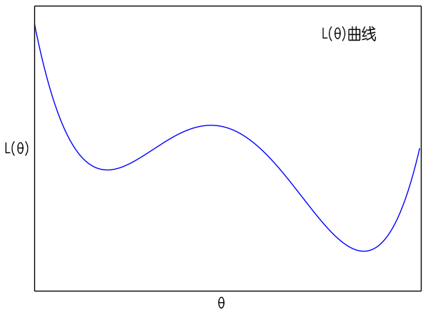 L(θ) curve
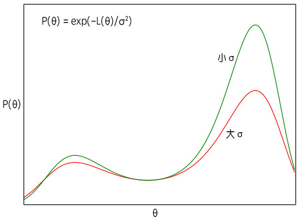 exp(-L(θ)) curve
Given this analysis, in theory, we should start with a smaller batch size, so that the noise variance $\sigma^2$ is larger and the distribution closer to uniform, allowing the algorithm to explore more of the region. As the number of iterations increases, we gradually approach the optimal region, and at that point the variance should decrease so that the extremum points become more prominent. In other words, if possible, the batch size should slowly increase as iterations proceed. This partially explains the result Google proposed last year in "Don't Decay the Learning Rate, Increase the Batch Size"], though increasing batch size substantially raises computational cost, so in practice we usually stop increasing it once it reaches a certain level.
Also, as we can see from the figure, once we enter the region of stable descent, the step size $\gamma$ (learning rate) per iteration should not exceed the width of the "pit," and the smaller $\sigma^2$ is, the narrower the pit becomes — this also suggests the learning rate should decrease as the number of iterations increases. Additionally, a larger $\gamma$ also partly introduces noise, so decreasing $\sigma^2$ in effect also means we should lower the learning rate.
So the conclusion of this analysis is:
Conditions permitting, when using SGD, start with a small batch size and a large learning rate, then let the batch size gradually increase while the learning rate gradually decreases.
As for the specific strategy for increasing or decreasing them, that's a matter of your own "model-training alchemy" skill.
Momentum Acceleration
As is well known, compared to adaptive learning-rate algorithms like Adam, plain SGD optimization is quite slow, and introducing momentum can accelerate SGD's convergence. This too has an elegant dynamical explanation.
From first order to second order
From the discussion above, we know that SGD and GD have essentially the same iteration scheme, so to find a way to accelerate SGD, we just need to find a way to accelerate GD, and then replace the full-batch gradient with the stochastic gradient. From the derivation from equation $(2)$ to equation $(4)$, we know that GD turns the problem of minimizing $L(\boldsymbol{\theta})$ into the problem of solving the ODE $\dot{\boldsymbol{\theta}} = - \nabla_{\boldsymbol{\theta}} L(\boldsymbol{\theta})$.
So, does it have to be first order? What about a second-order version $\ddot{\boldsymbol{\theta}} = - \nabla_{\boldsymbol{\theta}} L(\boldsymbol{\theta})$?
To this end, let's consider the general form
$$\ddot{\boldsymbol{\theta}} + \lambda \dot{\boldsymbol{\theta}} = - \nabla_{\boldsymbol{\theta}} L(\boldsymbol{\theta})\tag{10}$$
This truly corresponds to a (Newtonian) mechanical system, where $\lambda > 0$ introduces something like a frictional force. Let's analyze how such a system differs from the original first-order ODE of GD, $(4)$ and $(10)$.
First, from the perspective of fixed points: the stable fixed point that $(10)$ eventually converges to (where $\ddot{\boldsymbol{\theta}}=\dot{\boldsymbol{\theta}}=0$) is indeed a local minimum of $L(\boldsymbol{\theta})$. Imagine a ball rolling down from the top of a hill — it will naturally roll into a valley and then up again, but due to frictional resistance, it will eventually settle in the valley. Note that unless the algorithm never terminates, once it does stop, it must be at a valley (it could in principle be a peak or a saddle point, but these are low-probability outcomes) — it can never stop halfway up a slope, because there, potential energy still remains, and by conservation of energy it can be converted into kinetic energy, so the motion cannot stop.
Therefore, in terms of convergence behavior, this should be no different from first-order GD, so we only need to compare their convergence speeds.
GD + Momentum
We can rewrite $(10)$ equivalently as
$$\dot{\boldsymbol{\theta}}=\boldsymbol{\eta},\quad \dot{\boldsymbol{\eta}}=-\lambda \boldsymbol{\eta} - \nabla_{\boldsymbol{\theta}} L(\boldsymbol{\theta})\tag{11}$$
Discretizing $\dot{\boldsymbol{\theta}}$ gives
$$\dot{\boldsymbol{\theta}}\approx \frac{\boldsymbol{\theta}_{n+1}-\boldsymbol{\theta}_{n}}{\gamma}\tag{12}$$
So how should we handle $\boldsymbol{\eta}$? Should it be $\boldsymbol{\eta}_n$? No, no — $(\boldsymbol{\theta}_{n+1}-\boldsymbol{\theta}_{n})/\gamma$, taken as the derivative at time $n$, is only a first-order approximation ($\mathcal{O}(\gamma)$), whereas as the derivative at time $n+1/2$ it is a second-order approximation ($\mathcal{O}(\gamma^2)$). So, more precisely, we have:
$$\frac{\boldsymbol{\theta}_{n+1}-\boldsymbol{\theta}_{n}}{\gamma}=\boldsymbol{\eta}_{n+1/2}\tag{13}$$
Similarly, from the second equation of $(11)$, we derive the following result, which also has second-order accuracy:
$$\frac{\boldsymbol{\eta}_{n+1/2}-\boldsymbol{\eta}_{n-1/2}}{\gamma}=-\lambda\left(\frac{\boldsymbol{\eta}_{n+1/2}+\boldsymbol{\eta}_{n-1/2}}{2}\right)- \nabla_{\boldsymbol{\theta}} L(\boldsymbol{\theta}_n)\tag{14}$$
In short, for the sake of higher accuracy, $(\boldsymbol{\theta}_{n+1}-\boldsymbol{\theta}_{n})/\gamma$ is the derivative of $\boldsymbol{\theta}$ at time $n+1/2$, $(\boldsymbol{\eta}_{n+1/2}-\boldsymbol{\eta}_{n-1/2})/\gamma$ is the derivative of $\boldsymbol{\eta}$ at time $n$, and $(\boldsymbol{\eta}_{n+1/2}+\boldsymbol{\eta}_{n-1/2})/2=\boldsymbol{\eta}_n$. Both have accuracy of order $\mathcal{O}(\gamma^2)$.
Let
$$\boldsymbol{v}_{n+1}=\gamma\boldsymbol{\eta}_{n+1/2},\quad \beta = \frac{1-\lambda\gamma/2}{1+\lambda\gamma/2},\quad \alpha = \frac{\gamma^2}{1+\lambda\gamma/2}\tag{15}$$
Then combining with $(13),(14)$ we obtain
$$\begin{aligned}&\boldsymbol{\theta}_{n+1} = \boldsymbol{\theta}_{n} + \boldsymbol{v}_{n+1} \\ & \boldsymbol{v}_{n+1} = \beta\boldsymbol{v}_{n} - \alpha \nabla_{\boldsymbol{\theta}} L(\boldsymbol{\theta}_n) \end{aligned}\tag{16}$$
This is exactly GD with Momentum. Mathematically, it also has a special name: the "leapfrog integration method."
How does the acceleration work?
Combining equations $(15)$ and $(16)$, we can see how Momentum accelerates GD.
In GD's $(2)$, the learning rate is $\gamma$, the step size is also $\gamma$, and the accuracy is $\mathcal{O}(\gamma)$; in Momentum, the learning rate is $\alpha\approx \gamma^2$, the step size is $\gamma$, and the accuracy is $\mathcal{O}(\gamma^2)=\mathcal{O}(\alpha)$. Thus, once a learning rate $\alpha$ is fixed, at the same order of accuracy, Momentum actually advances with step size $\sqrt{\alpha}$, while plain GD advances with step size $\alpha$.
Since the learning rate is typically less than 1, we have $\sqrt{\alpha} > \alpha$. Hence:
One of the reasons Momentum accelerates convergence is that, for the same learning rate and without sacrificing accuracy, it lets the algorithm advance with a larger step size.
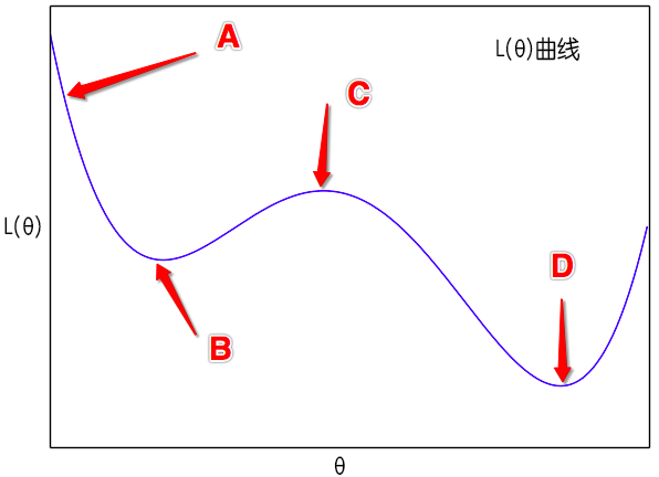 Starting from point A, sgd+momentum can reach point D, while sgd usually only reaches point B
Moreover, as shown in the figure, if we start from point $A$, gradient descent will gradually decrease down to point $B$ and eventually settle at point $C$. Of course, if the noise or the learning rate is large enough, it might overshoot past point $C$ and reach point $D$. But once we've added momentum, $(10)$ becomes a dynamical equation, and everything from Newtonian mechanics applies here. Starting from point $A$ with zero initial velocity, it slowly descends, converting potential energy into kinetic energy; then after passing through point $B$, it slowly rises again, converting kinetic energy back into potential energy. If the friction is small, then upon reaching point $C$ there is still kinetic energy left, and it can go directly on to reach point $D$. This is guaranteed by conservation of energy, even without noise. In plain SGD, achieving a similar effect requires a large learning rate and small batch size (i.e., stronger noise).
So we can also say:
Momentum acceleration provides a dynamical mechanism for "jumping over" less desirable local minima.
So how should $\lambda$ be chosen? Can't we simply set $\lambda=0$ or $\beta=1$?
As mentioned earlier, the term $\lambda > 0$ acts like friction, dissipating energy. Without this term, no matter how small the learning rate is — as long as it's not zero — the Momentum algorithm will never settle at a minimum; it will keep moving forever. It's like a pendulum without friction: it will keep swinging without stopping, as guaranteed by conservation of energy. Energy conservation tells us that at the lowest point of the energy landscape (i.e., our desired minimum), the kinetic energy — and hence speed — is at its maximum. In other words, the algorithm simply can't stop! But if friction dissipates energy so that energy is no longer conserved, then the pendulum eventually comes to rest at the lowest point. So introducing $\lambda$ is necessary for the algorithm's convergence, and from $(15)$ we have $\beta < 1$. However, $\lambda$ also cannot be too large — excessive friction will cause the motion to stop before reaching the minimum. To ensure the acceleration effect still holds, we also need $\beta > 0$.
Finally, from the definition of $\beta$ in equation $(15)$, we can see that when $\lambda$ is fixed (i.e., the friction coefficient is fixed), if the learning rate $\alpha$ decreases (implying $\gamma$ also decreases), then $\beta$ should increase correspondingly, and the proportion of the increase can be roughly estimated. From $(15)$ we get the approximation $1-\lambda\sqrt{\alpha}=\beta$, from which we can back out $\lambda$; then, substituting the new $\alpha$, we can compute the new $\beta$.
This gives us a reference tuning scheme for $\beta$ in an SGD+Momentum optimizer:
When using SGD+Momentum, if you lower the learning rate, you should slightly raise $\beta$. When the learning rate drops from $\alpha$ to $r\alpha$, $\beta$ can be considered for an increase up to $1 - (1-\beta)\sqrt{r}$.
Nesterov Momentum
The Momentum algorithm is essentially numerically solving $(10)$, and solving $(10)$ doesn't have to use the explicit iteration scheme $(13),(14)$ — an implicit iteration scheme is also possible. For instance, we can approximate $(10)$ as
$$\begin{aligned}&\frac{\boldsymbol{\theta}_{n+1}-\boldsymbol{\theta}_{n}}{\gamma} = \frac{\boldsymbol{\eta}_{n+1}+\boldsymbol{\eta}_{n}}{2}\\ &\frac{\boldsymbol{\eta}_{n+1}-\boldsymbol{\eta}_{n-1}}{2\gamma} = -\lambda \frac{\boldsymbol{\eta}_{n}+\boldsymbol{\eta}_{n-1}}{2} - \nabla_{\boldsymbol{\theta}} L\left(\frac{\boldsymbol{\theta}_{n+1}+\boldsymbol{\theta}_n}{2}\right) \end{aligned}\tag{17}$$
Letting
$$\boldsymbol{v}_{n+1}=\frac{\gamma}{2}(\boldsymbol{\eta}_{n+1}+\boldsymbol{\eta}_{n}),\quad \beta = 1-\lambda\gamma,\quad \alpha=\gamma^2\tag{18}$$
we obtain
$$\begin{aligned}&\boldsymbol{\theta}_{n+1} = \boldsymbol{\theta}_{n} + \boldsymbol{v}_{n+1} \\ & \boldsymbol{v}_{n+1} = \beta\boldsymbol{v}_{n} - \alpha \nabla_{\boldsymbol{\theta}} L\left(\frac{\boldsymbol{\theta}_{n+1}+\boldsymbol{\theta}_n}{2}\right) \end{aligned}\tag{19}$$
This is an implicit iterative formula; in principle, solving for $\boldsymbol{\theta}_{n+1}$ would require solving a nonlinear system of equations. But as an approximation, we only need to approximate $\boldsymbol{\theta}_{n+1}$ with $\boldsymbol{\theta}_{n}+\beta \boldsymbol{v}_{n}$, yielding
$$\begin{aligned}&\boldsymbol{\theta}_{n+1} = \boldsymbol{\theta}_{n} + \boldsymbol{v}_{n+1} \\ & \boldsymbol{v}_{n+1} = \beta\boldsymbol{v}_{n} - \alpha \nabla_{\boldsymbol{\theta}} L\left(\boldsymbol{\theta}_n + \frac{\beta}{2}\boldsymbol{v}_n\right) \end{aligned}\tag{20}$$
If we replace $\beta/2$ inside the parentheses with $\beta$, then this becomes the standard GD algorithm with Nesterov momentum. However, I think the equation above seems more sensible, because the Nesterov algorithm tries to substitute the gradient at $\boldsymbol{\theta}_{n+1}$ for the gradient at $\boldsymbol{\theta}_n$, giving the algorithm "look-ahead capability" — but in fact this is still somewhat biased, and intuitively using the gradient at $(\boldsymbol{\theta}_n+\boldsymbol{\theta}_{n+1})/2$ feels more balanced.
From the point of view of error analysis, whether it's the standard Momentum or the Nesterov version, both are second-order algorithms with the same accuracy (differing only by a constant factor). But theoretically, Nesterov is an implicit iteration with a wider region of stability, so it usually achieves better results in practice.
How would we implement equation $(20)$ in a framework like TensorFlow? Note that $(20)$ involves first differentiating $L(\boldsymbol{\theta})$ with respect to $\boldsymbol{\theta}$, and then substituting $\boldsymbol{\theta}$ with $\boldsymbol{\theta}_n + \frac{\beta}{2}\boldsymbol{v}_n$ (my version here) or $\boldsymbol{\theta}_n + \beta\boldsymbol{v}_n$ (the standard Nesterov). This operation may seem simple to us, but it's rather cumbersome to implement in frameworks like TensorFlow.
The reason is that although these frameworks support automatic differentiation, they are ultimately numerical computation frameworks rather than symbolic computation systems, so the result is just a numerical derivative. Once we've computed the derivative of $\boldsymbol{\theta}$, the result is a tensor — some fixed numbers — and substituting $\boldsymbol{\theta}$ with $\boldsymbol{\theta}_n + \frac{\beta}{2}\boldsymbol{v}_n$ becomes rather awkward. It's not impossible, of course, but it's certainly not as straightforward as the one-step Momentum version.
So, for ease of implementation, we set (taking the standard Nesterov as an example):
$$\boldsymbol{\Theta}_n=\boldsymbol{\theta}_n + \beta\boldsymbol{v}_n$$
which gives us a new iterative formula:
$$\begin{aligned}&\boldsymbol{\Theta}_{n+1} = \boldsymbol{\Theta}_{n} + \beta\boldsymbol{v}_{n+1} - \alpha \nabla_{\boldsymbol{\theta}} L\left(\boldsymbol{\Theta}_n\right) \\ & \boldsymbol{v}_{n+1} = \beta\boldsymbol{v}_{n} - \alpha \nabla_{\boldsymbol{\theta}} L\left(\boldsymbol{\Theta}_n\right) \end{aligned}$$
This is how mainstream frameworks implement the Nesterov algorithm — for instance, Keras's ] — which avoids the need for variable substitution. As iterations get closer and closer to the minimum, the momentum $\boldsymbol{v}$ becomes smaller and smaller, so $\boldsymbol{\Theta}$ and $\boldsymbol{\theta}$ will eventually become equivalent — even if there is some small discrepancy, it doesn't matter much, since the whole point of using momentum is acceleration, and model selection is based on performance on the validation set anyway.
The Kramers Equation
The discussion so far has only covered momentum acceleration for full-batch gradient descent. Finally, let's briefly analyze the case of stochastic gradient descent. Under the same assumptions as before, introducing the stochastic gradient means that $(10)$ becomes an equation with a random force:
$$\ddot{\boldsymbol{\theta}} + \lambda \dot{\boldsymbol{\theta}} = - \nabla_{\boldsymbol{\theta}} L(\boldsymbol{\theta})+\sigma\boldsymbol{\xi}\tag{21}$$
This is called the "Kramers equation," and, like the Langevin equation, is a central result in stochastic dynamics. When $\lambda=0$, the static solution can be written down explicitly, and this static distribution can serve as a reference in the general case:
$$P(\boldsymbol{\theta},\boldsymbol{\eta}) \sim \exp\left(-\frac{\boldsymbol{\eta}^2/2 + L(\boldsymbol{\theta})}{\sigma^2}\right)\tag{22}$$
where $\boldsymbol{\eta}=\dot{\boldsymbol{\theta}}$, and the marginal distribution of $\boldsymbol{\theta}$ is exactly given by equation $(9)$. So we can consider that the earlier analysis for plain SGD carries over equally to the Momentum and Nesterov algorithms.
Reflections
This article aims to analyze aspects of SGD from a dynamical-systems perspective. It cannot give precise answers to the questions raised at the beginning of the article, but I hope it offers some useful intuition. Although this piece is rather long and equation-heavy, readers with an undergraduate background in numerical computation should not find it too hard to follow. If you have any questions, feel free to leave a comment and let's discuss further.
Translated automatically with claude-sonnet-5; all equations are reproduced verbatim from the source. Copyright remains with the original author.