Cutting Through the Mist: A Delicious Feast of Capsules
 Geoffrey Hinton at Google's Toronto office
The Capsule paper Dynamic Routing Between Capsules, open-sourced by deep learning pioneer Hinton, was without doubt one of the hottest topics in the deep learning world last year. Thanks to all kinds of media hype, Capsule was crowned with a mysterious aura, with phrases like "abandons gradient descent" and "reinvents deep learning from scratch" popping up everywhere. But some people also feel that Capsule is nothing more than a new buzzword.
This post attempts to cut through the confusing mist and get to grips with the principles and appeal behind Capsule, so that we can savor this feast properly. Along the way, I've also run an experiment of my own design — one that, I think, demonstrates the effectiveness of Capsule more convincingly than the experiments in the original paper.
Menu overview:
1. What is Capsule?
2. Why is Capsule designed this way?
3. Is Capsule really any good?
4. What do I think of Capsule?
5. A few side dishes.
Preface
The Capsule paper has been out for a few months now, and there are already plenty of great write-ups online, as well as open-source CapsuleNet implementations, all of which have sped up my own understanding of Capsule. However, I feel that most of the online explanations fall a bit short: they merely dress up a translation of the paper with a bit of extra phrasing, without really explaining the principles behind Capsule. Take the "dynamic routing" section, for example — most write-ups just copy the algorithm from the paper verbatim and then note that it converges after 3 iterations. But converges to what? The paper doesn't say, and neither do the write-ups. This is clearly unsatisfying. It's no wonder a reader on Zhihu commented:
The so-called capsule is just another flashy trick dressed up as a contribution to deep learning. I call it a trick because Hinton never explains why the routing algorithm needs exactly that many steps, with loops nested inside loops — is there any theoretical basis, or was it just cobbled together?
That comment may be a bit harsh, but it does hit the mark: why should we just blindly follow along with an algorithm Hinton has laid out, with no explanation given?
The Capsule Feast
The Special Feature of the Feast
The special feature of this Capsule feast is "vector in, vector out," replacing the old "scalar in, scalar out" paradigm — that is, the inputs and outputs of a neuron become vectors, which is touted as a revolution in neural network theory. But is that really so? Haven't we already been doing "vector in, vector out" tasks all along? Yes, plenty of them! In NLP, isn't a sequence of word embeddings fed in already a "vector in"? And after being encoded by an RNN/CNN/Attention module, doesn't that sequence become a "vector out"? In today's deep learning, examples of "vector in, vector out" are never in short supply, so this clearly can't be counted as Capsule's revolution.
Capsule's revolution lies elsewhere: it proposes a new scheme for propagating "vector in, vector out" information, and this scheme is, to a large extent, interpretable.
If asked why deep learning (neural networks) works, I would generally answer this way: neural networks perform layer-by-layer abstraction of the input through stacked layers, a process that to some extent mimics how humans perform hierarchical classification, ultimately producing the final output with reasonably good generalization. Indeed, neural networks probably do work this way — but they can't actually tell us that this is precisely what's happening, and that's the source of neural networks' notorious lack of interpretability, which is one reason many people regard deep learning as a black box.
Let's see how Hinton tries to break through this limitation with Capsule.
The Grand Basin Feast
If I had to use a dish to describe Capsule, I'd think of "poon choi" (盆菜), the Cantonese "big basin feast":
Poon choi, as a Hakka dish, has a long history — it's also commonly known as "the great platter dish." It originates from the traditional Hakka "prosperity platter": as the name suggests, you take one big plate and pile all the food into it, letting the flavors mingle into something uniquely delicious. Rich ingredients are layered one on top of another into the big basin, with the ingredients that most readily absorb the sauce typically placed at the bottom. When eating, each table gets one basin, and you eat your way down layer by layer, as the juices intermingle and the flavor grows richer and more fragrant, giving diners the delightful sense of gradually entering ever more exquisite territory.
Capsule is designed with precisely this "layer-by-layer progression" goal in mind. But frankly, the writing in the Capsule paper leaves much to be desired, so in this post I'll try to avoid reusing the paper's notation as much as possible, to spare readers further confusion. Let's look at a diagram.
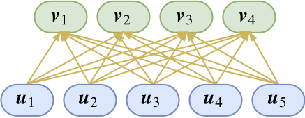 Capsule diagram
As shown in the figure, the lower-level capsules and the higher-level capsules form a set of connections. Wait — what exactly is a "capsule"? Actually, all you need to do is treat a vector as a single unit, and that's a "capsule." Yes, you read that right — you can think of it this way: a neuron is a scalar, a capsule is a vector, that's really all there is to it! Hinton's own understanding is: each capsule represents an attribute, and the capsule's vector represents a "frame" for that attribute. In other words, whereas before we only used a scalar to indicate whether a feature was present or not (e.g., whether there are feathers), now we use a vector to represent not just whether it's present, but also "what kind" it is (e.g., what color or texture of feathers). Understood this way, this means the representation of a single feature has become richer.
This reminds me a bit of word embeddings in NLP: previously, we only used one-hot encoding to represent a word, which merely indicated whether that word was present or not. Now we use word embeddings to represent a word, and clearly word embeddings carry richer features — not only indicating presence but also which words have similar meanings. Are word embeddings the "capsules" of NLP? The analogy might be a bit of a stretch, but I think the underlying idea is right.
So, how should these capsules be combined so as to embody the properties of "layer-by-layer abstraction" and "layer-by-layer classification"? Let's first look at part of the connections:
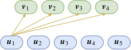 Take a closer look at part of the capsule's connections
The figure only shows the connections for $\boldsymbol{u}_1$. That is to say, we already have the feature $\boldsymbol{u}_1$ (say, feathers), and we want to know which of the higher-level features $\boldsymbol{v}_1,\boldsymbol{v}_2,\boldsymbol{v}_3,\boldsymbol{v}_4$ (say, representing chicken, duck, fish, and dog respectively) it belongs to. This is obviously a classification problem we're already quite familiar with — isn't it just an inner product followed by softmax? So, based on the single feature $\boldsymbol{u}_1$ alone, we derive that the probabilities of it belonging to chicken, duck, fish, and dog respectively are
$$\big(p_{1|1},p_{2|1},p_{3|1},p_{4|1}\big) = \frac{1}{Z_1}\Big(e^{\langle\boldsymbol{u}_1,\boldsymbol{v}_1\rangle}, e^{\langle\boldsymbol{u}_1,\boldsymbol{v}_2\rangle}, e^{\langle\boldsymbol{u}_1,\boldsymbol{v}_3\rangle}, e^{\langle\boldsymbol{u}_1,\boldsymbol{v}_4\rangle}\Big)\tag{1}$$
Naturally, we would expect $p_{1|1}$ and $p_{2|1}$ to be noticeably larger than $p_{3|1}$ and $p_{4|1}$. However, relying on this single feature alone isn't enough — we need to combine information across multiple features, so we can perform the same operation for each $\boldsymbol{u}_i$, obtaining $\big(p_{1|2},p_{2|2},p_{3|2},p_{4|2}\big)$, $\big(p_{1|3},p_{2|3},p_{3|3},p_{4|3}\big)$, and so on.
The problem is, now that we have all these prediction results, which one should we pick? And actually, we're not really trying to do classification here — what we want is to fuse these features together into a higher-level feature. So Hinton's idea is: since the feature $\boldsymbol{u}_i$ yields the probability distribution $\big(p_{1|i},p_{2|i},p_{3|i},p_{4|i}\big)$, we can split this feature into four parts, namely $\big(p_{1|i}\boldsymbol{u}_i,p_{2|i}\boldsymbol{u}_i,p_{3|i}\boldsymbol{u}_i,p_{4|i}\boldsymbol{u}_i\big)$, and pass these parts respectively to $\boldsymbol{v}_1,\boldsymbol{v}_2,\boldsymbol{v}_3,\boldsymbol{v}_4$. Then $\boldsymbol{v}_1,\boldsymbol{v}_2,\boldsymbol{v}_3,\boldsymbol{v}_4$ is simply the sum of the features passed up from each of the lower-level capsules — wouldn't that work nicely?
$$\boldsymbol{v}_j = squash\left(\sum_{i} p_{j|i} \boldsymbol{u}_i\right) = squash\left(\sum_{i} \frac{e^{\langle\boldsymbol{u}_i,\boldsymbol{v}_j\rangle}}{Z_i} \boldsymbol{u}_i\right)\tag{2}$$
Viewed from top to bottom, Capsule has each lower-level feature perform its own classification, and then integrates the classification results. In this process, $\boldsymbol{v}_j$ should stay as close as possible to all of the $\boldsymbol{u}_i$, where closeness is measured by inner product. So, viewed from bottom to top, we can regard $\boldsymbol{v}_j$ as essentially a kind of cluster center for the various $\boldsymbol{u}_i$, and the core idea of Capsule is that the output is some kind of clustering result of the inputs.
Now let's look at what this $squash$ actually is, and where it comes from.
Concentrated Juice
The word "squash" in English also carries the sense of concentrated juice, so let's think of it as a glass of juice to be savored. This "juice" arises because Hinton wanted Capsule to have the property that the length (norm) of a capsule vector represents the probability of that feature.
Actually, I'm not fond of the term "probability" here, because probability makes us think of normalization, and normalization is in fact a rather troublesome thing. I think it's better described as the "salience" of the feature — this is easier to explain: the larger the norm, the more salient the feature. And we want a bounded indicator to measure this "salience," so we're forced to compress this norm — after all, "concentration is the essence." The compression scheme Hinton chose is:
$$squash(\boldsymbol{x})=\frac{\Vert\boldsymbol{x}\Vert^2}{1+\Vert\boldsymbol{x}\Vert^2}\frac{\boldsymbol{x}}{\Vert\boldsymbol{x}\Vert}\tag{3}$$
The $\boldsymbol{x}/\Vert\boldsymbol{x}\Vert$ part is easy to understand — it just normalizes the vector to unit length. But how should we understand the first part? Why choose it this way? In fact, there are many possible schemes for compressing a norm into the range 0–1, for example:
$$\tanh \Vert\boldsymbol{x}\Vert, \quad 1-e^{-\Vert\boldsymbol{x}\Vert}, \quad \frac{\Vert\boldsymbol{x}\Vert}{1+\Vert\boldsymbol{x}\Vert}$$
and so on — it's not clear what line of reasoning led Hinton to pick the particular scheme he did. Perhaps each scheme is worth exploring on its own? In fact, in some of my own experiments, I found that choosing
$$squash(\boldsymbol{x})=\frac{\Vert\boldsymbol{x}\Vert^2}{0.5+\Vert\boldsymbol{x}\Vert^2}\frac{\boldsymbol{x}}{\Vert\boldsymbol{x}\Vert}$$
works a bit better. The distinguishing feature of this function is that it amplifies values when the norm is very close to 0, rather than uniformly compressing everything as the original function does.
That said, one question worth pondering is: in the intermediate layers, is this squashing operation actually necessary? Since dynamic routing (discussed below) is already present, the network already has nonlinearity even without the $squash$ function, so intuitively there's no real need to apply feature compression in the intermediate layers either — just as ordinary neural networks don't necessarily need a sigmoid function to squash values into 0–1. I think this deserves careful empirical testing.
Dynamic Routing
Notice that in equation $(2)$, computing $\boldsymbol{v}_j$ requires a softmax, but computing that softmax in turn requires knowing $\boldsymbol{v}_j$ — isn't this a chicken-and-egg problem? This is where the "main course" comes in: "Dynamic Routing," which can update (some of) the parameters based on its own internal dynamics, thereby taking a first step toward Hinton's goal of doing away with gradient descent.
But is this "main course" really what it appears to be? How was it conceived? What does it ultimately converge to? Let's first sample two side dishes, and then slowly savor the main course.
Side Dish 1
Let's go back to an ordinary neural network. As we know, the activation function plays a pivotal role in a neural network. Of course, the activation function itself is simple — for example, a tanh-activated fully connected layer, written in TensorFlow, looks like this:
y = tf.matmul(W, x) + b
y = tf.tanh(y)
But what if I wanted to use the inverse function of $x = y + \cos y$ as the activation? That is, you'd need to solve for $y=f(x)$ and then use that as the activation function.
Mathematicians tell us, however, that the inverse function here is a transcendental function — meaning it cannot be expressed in a finite closed form using elementary functions. Isn't that just deliberately awkward? Not a problem — we have iteration:
$$y_{n+1}=x-\cos y_n$$
Choose $y_0 = x$, substitute it into the above equation, and iterate a few times, and you'll get a reasonably accurate value of $y$. If we iterate three times, we get
$$y=x-\cos\big(x-\cos(x-\cos x)\big)$$
Written in TensorFlow, this becomes
y = tf.matmul(W, x) + b
Y = y
for i in range(3):
    Y = y - tf.cos(Y)
If readers have already "previewed" Capsule, they'll notice this looks very much like Capsule's dynamic routing.
Side Dish 2
Let's look at another example — one that has plenty of counterparts in NLP, though it's not uncommon in vision either. Consider a sequence of vectors $(\boldsymbol{x}_1,\boldsymbol{x}_2,\dots,\boldsymbol{x}_n)$. I now want to find a way to combine these $n$ vectors into a single vector $\boldsymbol{x}$ (an encoder), and then use that vector for classification.
Readers might think of using an LSTM here. But what I want is simply to express it as a linear combination of the original vectors, that is:
$$\boldsymbol{x}=\sum_{i=1}^{n} \lambda_i \boldsymbol{x}_i$$
Here, $\lambda_i$ effectively measures the similarity between $\boldsymbol{x}$ and $\boldsymbol{x}_i$. But here's the problem: before $\boldsymbol{x}$ even exists, how can we possibly determine this similarity? Isn't this also a chicken-and-egg problem? One solution is, again, iteration. First, we can define a softmax-based similarity measure, and then let
$$\boldsymbol{x}=\sum_{i=1}^{n} \frac{e^{\langle\boldsymbol{x},\boldsymbol{x}_i\rangle}}{Z} \boldsymbol{x}_i$$
At the start, we know nothing, so we simply take $\boldsymbol{x}$ to be the average of all the $\boldsymbol{x}_i$, substitute it into the right-hand side to compute a $\boldsymbol{x}$, then substitute that back in, and repeat — this iteration generally converges after a finite number of steps, and so this iterative process can be embedded directly into the neural network.
If Side Dish 1 only resembled dynamic routing in spirit, then Side Dish 2 resembles it both in spirit and in form. That said, I haven't seen any existing work that does exactly this — this side dish is purely a brainstorm of my own.
The main course
With those two side dishes out of the way, the dynamic routing "main course" is really not mysterious at all. To obtain each $\boldsymbol{v}_j$, we simply start by setting all of them equal to the mean of $\boldsymbol{u}_i$, and then iterate repeatedly. In plain terms, the output is the result of clustering the input, and clustering usually requires an iterative algorithm — that iterative algorithm is called "dynamic routing." As for the specific details of this dynamic routing, they are not fixed; they depend on the clustering algorithm being used. For instance, the newer Capsule paper MATRIX CAPSULES WITH EM ROUTING uses a Gaussian Mixture Model for clustering.
With this understanding, we can now write down this post's version of the dynamic routing algorithm:
Dynamic Routing Algorithm
Initialize $b_{ij}=0$
Iterate $r$ times:
$\boldsymbol{c}_i \leftarrow softmax(\boldsymbol{b}_i)$;
$\boldsymbol{s}_j \leftarrow \sum\limits_i c_{ij} \boldsymbol{u}_i$;
$\boldsymbol{v}_j \leftarrow squash(\boldsymbol{s}_j)$;
$b_{ij} \leftarrow \langle\boldsymbol{u}_i,\boldsymbol{v}_j\rangle$.
Return $\boldsymbol{v}_j$.
Here $c_{ij}$ is the same as $p_{j|i}$ from earlier.
"Hey, finally caught you in a mistake! I've read the paper — shouldn't it be $b_{ij} \leftarrow b_{ij} + \langle\boldsymbol{u}_i,\boldsymbol{v}_j\rangle$ rather than $b_{ij} \leftarrow \langle\boldsymbol{u}_i,\boldsymbol{v}_j\rangle$?"
Actually, the algorithm above is not wrong — if you accept this post's derivation, and accept equation $(2)$, then the iteration above is correct.
"You mean Hinton got it wrong? And you think you're qualified to challenge Hinton?" Hold on, hold on — let me first walk through what goes wrong in Hinton's iteration. If we follow Hinton's algorithm, then we have $b_{ij} \leftarrow b_{ij} + \langle\boldsymbol{u}_i,\boldsymbol{v}_j\rangle$, so after $r$ iterations, it becomes:
$$\boldsymbol{v}_j^{(r)}=squash\left(\sum_i\frac{e^{\big\langle\boldsymbol{u}_{i},\,\boldsymbol{v}_{j}^{(0)}+\boldsymbol{v}_{j}^{(1)}+\dots+\boldsymbol{v}_{j}^{(r-1)}\big\rangle}}{Z_i}\boldsymbol{u}_{i}\right)$$
Since $\boldsymbol{v}_j^{(r)}$ will keep getting closer to the true $\boldsymbol{v}_j$, we can write
$$\boldsymbol{v}_j^{(r)}\sim squash\left(\sum_i\frac{e^{r\langle\boldsymbol{u}_{i},\,\boldsymbol{v}_j\rangle}}{Z_i}\boldsymbol{u}_{i}\right)$$
If we iterate infinitely many times (in practice this is impossible due to limited compute, but it's theoretically always achievable), then $r\to\infty$, so that the softmax output becomes either exactly 0 or exactly 1. In other words, each lower-level capsule ends up connected to exactly one upper-level capsule.
Is that reasonable? I don't think so. Different categories can very well share common features — cats and dogs are different, but they both have roughly similar eyes. Some readers have explained this issue by saying: $r$ is a hyperparameter, and it shouldn't be too large, since making it too large leads to overfitting. First, I don't know whether Hinton actually had this in mind, but I believe that treating $r$ as a hyperparameter makes Capsules far too ugly!
Indeed — dynamic routing has already been criticized by many readers as "incomprehensible." If on top of that we add a hyperparameter that goes against intuition, wouldn't that make it even uglier? By contrast, if we instead start from this post's equation $(2)$ and derive the dynamic routing algorithm presented here, the result matches the spirit of clustering and looks theoretically nicer, since in this case $r$ simply benefits from being as large as possible (limited only by available compute) — there's no such hyperparameter involved. In fact, after making this modification, I ran it on the currently open-sourced Capsule code and got the same results.
As for which version readers choose to adopt, that's up to them. Personally, I have a bit of a perfectionist streak and can't stand theoretical loose ends.
Model Details
Below I describe the implementation details of Capsule. The corresponding code is on my Github, though currently only a Keras version is available. Compared to the previously implemented version, my version is implemented purely in Keras (the original was half Keras, half raw TensorFlow), and by replacing the author's use of K.map_fn with K.local_conv1d, I achieved a speedup of several times — this is because K.map_fn does not automatically parallelize, and to parallelize it you need to find a way to fold everything into a single matrix operation. Secondly, I implemented the shared-parameter version via K.conv1d. The code runs on Python 2.7 + TensorFlow 1.8 + Keras 2.1.4.
Fully Connected Version
Setting aside whether it's Hinton's version or mine, if $\boldsymbol{v}_j$ can simply be computed iteratively via this dynamic routing algorithm, doesn't that mean there are no parameters at all? Have we really done away with backpropagation?
Not at all! If that were really the case, then every $\boldsymbol{v}_j$ would end up identical. As mentioned earlier, $\boldsymbol{v}_j$ appears as a kind of clustering center for the input $\boldsymbol{u}_i$, and clearly, looking at the input from different angles produces different clustering results. So in order to achieve this "multi-angle view of features," we can multiply by a transformation matrix before passing each capsule on to the next one. So equation $(2)$ should actually become
$$\boldsymbol{v}_j = squash\left(\sum_{i} \frac{e^{\langle\hat{\boldsymbol{u}}_{j|i},\,\boldsymbol{v}_j\rangle}}{Z_i} \hat{\boldsymbol{u}}_{j|i}\right),\quad \hat{\boldsymbol{u}}_{j|i} = \boldsymbol{W}_{ji}\boldsymbol{u}_i\tag{4}$$
Here, $\boldsymbol{W}_{ji}$ is a trainable matrix, and the multiplication here is matrix multiplication, i.e., a matrix times a vector. So Capsule becomes what's shown in the diagram below.
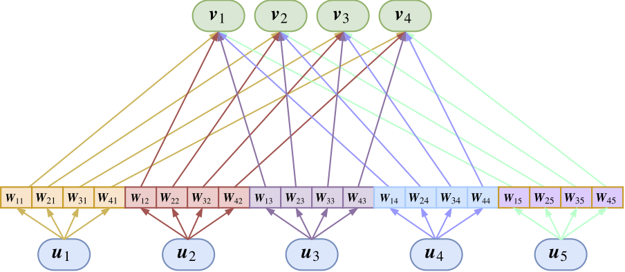 Diagram of the fully-connected version of Capsule
At this point we can write down the complete dynamic routing algorithm:
Dynamic Routing Algorithm
Initialize $b_{ij}=0$
Iterate $r$ times:
$\boldsymbol{c}_i \leftarrow softmax(\boldsymbol{b}_i)$;
$\boldsymbol{s}_j \leftarrow \sum\limits_i c_{ij} \hat{\boldsymbol{u}}_{j|i}$;
$\boldsymbol{v}_j \leftarrow squash(\boldsymbol{s}_j)$;
$b_{ij} \leftarrow \langle\hat{\boldsymbol{u}}_{j|i} , \boldsymbol{v}_j\rangle$.
Return $\boldsymbol{v}_j$.
A Capsule layer of this kind is clearly equivalent to a fully connected layer in an ordinary neural network.
Shared-Weight Version
As we all know, fully connected layers can only handle fixed-length inputs, and the fully-connected version of Capsule is no exception. But the images processed by CNNs are typically of varying size, so the number of extracted features is not fixed either — in this situation, the fully-connected Capsule layer no longer applies. As shown in the earlier figure, the number of transformation matrices equals the number of input capsules times the number of output capsules; since the number of inputs is not fixed, we cannot use a fully connected layer.
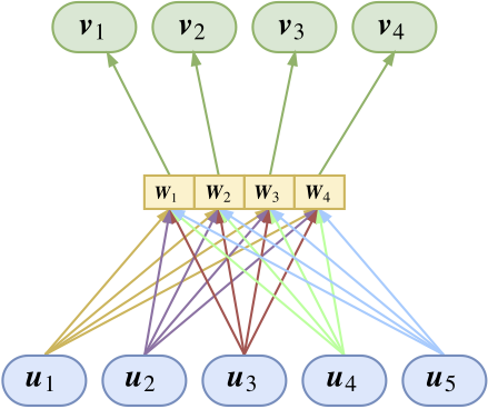 Parameter-shared version of Capsule
So, just like weight sharing in CNNs, we also need a weight-shared version of Capsule. What we mean by the "shared" version is: for a fixed upper-level capsule $j$, the transformation matrix connecting it to all lower-level capsules is shared, i.e., $\boldsymbol{W}_{ji}\equiv \boldsymbol{W}_j$.
As shown in the diagram, the shared version really isn't hard to understand: viewed bottom-up, all input vectors get mapped through the same matrix, then get clustered to produce an output; repeat this process a few times, and you get that many output vectors (capsules). Or viewed top-down, each transformation matrix can be seen as a detector belonging to the upper-level capsule, which the upper-level capsule uses to recognize whether the given feature is present in the lower-level capsule. So it's clear that this version's parameter count does not depend on the number of input capsules, and hence it can easily be attached right after a CNN. For the shared version, equation $(2)$ becomes
$$\boldsymbol{v}_j = squash\left(\sum_{i} \frac{e^{\langle\hat{\boldsymbol{u}}_{j|i},\boldsymbol{v}_j\rangle}}{Z_i} \hat{\boldsymbol{u}}_{j|i}\right),\quad \hat{\boldsymbol{u}}_{j|i} = \boldsymbol{W}_{j}\boldsymbol{u}_i\tag{5}$$
As for the dynamic routing algorithm, it remains unchanged.
Backpropagation
Although I'm not particularly fond of the term "backpropagation," it seems unavoidable here.
Now that we have $\boldsymbol{W}_{ji}$, how are these parameters trained? The answer is backpropagation. What might confuse readers is: now that we have both dynamic routing and backpropagation, how exactly do the two work together? Actually, this is about as simple as it gets. Just like in "side dish 1," we take the handful of iteration steps of the algorithm (3 steps in the paper) and fold them into the model. Formally speaking, this just means adding three extra layers to the model — everything else proceeds as usual, and in the end we build a loss to backpropagate through.
Seen this way, Capsule not only contains backpropagation, it contains nothing but backpropagation — because dynamic routing has already been absorbed into the model itself, and no longer counts as a separate iterative algorithm.
What Does It Actually Do
It's worth stepping back and asking: what does Capsule actually do? Put in the most direct terms, Capsule simply provides a new "vector in, vector out" scheme, which in that sense isn't so different from CNN, RNN, or attention layers. From Hinton's original intent, it provides a new scheme — based on the idea of clustering — for aggregating features in place of pooling, and this new scheme has stronger representational power.
Experiments
MNIST Classification
Unsurprisingly, Capsule was first tested on MNIST, where it performed quite well. By perturbing certain values inside a capsule and reconstructing the image, it was indeed found that these values encode some meaningful semantics — this shows that Capsule achieves, at least preliminarily, its stated goal.
The way Capsule is used for classification differs from ordinary neural networks in that: Capsule ultimately outputs 10 vectors (i.e., 10 capsules), each representing one class, and the norm of each vector represents its probability. In fact, what Capsule is doing is detecting the presence or absence of each class — that is, it converts a multi-class classification problem into multiple binary classification problems. Because of this, it does not use ordinary cross-entropy loss, but instead uses
$$L_c = T_c \max(0, m^+ − \Vert \boldsymbol{v}_c\Vert)^2 + \lambda (1 − T_c) \max(0, \Vert \boldsymbol{v}_c\Vert − m^−)^2$$
where $T_c$ is either 0 or 1, indicating whether the sample belongs to that class. Of course, there's nothing particularly special about this choice — several alternatives would work too. The paper also compares the improvement obtained by adding a reconstruction network.
Overall, the experiments in the paper feel a bit rough — choosing MNIST for the experiments seems a bit underwhelming (they could at least have tried Fashion-MNIST), and the reconstruction network is also just a crude stack of two fully connected layers. That said, given the paper's purpose — just to demonstrate that the pipeline works — it's passable.
My Experiment
Since ordinary convolutional neural networks already achieve 99%+ validation accuracy on MNIST, simply claiming "Capsule works" on this basis wouldn't be very convincing. So here I designed a new experiment for Capsule. Although this experiment is still based on MNIST, it demonstrates quite convincingly that Capsule has a genuinely strong ability to integrate features. Capsule doesn't just work — it works beautifully.
The experiment is set up as follows:
1. Using the existing MNIST dataset, train a digit-recognition model, but instead of using softmax for 10-way classification, convert it into 10 binary classification problems. Clearly, this can be done with either the old CNN+Pooling architecture or today's CNN+Capsule architecture.
2. After training the model, test it. But the test images are not the original test set — instead, we randomly pick two images from the test set and paste them together, then check whether the model can correctly predict both digits (as an unordered pair, order doesn't matter).
In other words, the training set is "one digit per image," while the test set is "two digits per image."
The experiment was implemented in Keras; the full code is available on my Github. Only the core parts are shown here.
First, the CNN. To keep things fair, everyone's CNN model is identical:
#CNN部分,这部分两个模型都一致
input_image = Input(shape=(None,None,1))
cnn = Conv2D(64, (3, 3), activation='relu')(input_image)
cnn = Conv2D(64, (3, 3), activation='relu')(cnn)
cnn = AveragePooling2D((2,2))(cnn)
cnn = Conv2D(128, (3, 3), activation='relu')(cnn)
cnn = Conv2D(128, (3, 3), activation='relu')(cnn)
We first model this with ordinary Pooling + fully connected layers:
cnn = GlobalAveragePooling2D()(cnn)
dense = Dense(128, activation='relu')(cnn)
output = Dense(10, activation='sigmoid')(dense)

model = Model(inputs=input_image, outputs=output)
model.compile(loss=lambda y_true,y_pred: y_true*K.relu(0.9-y_pred)**2 + 0.25*(1-y_true)*K.relu(y_pred-0.1)**2,
              optimizer='adam',
              metrics=['accuracy'])
This code has about 270,000 parameters, and reaches over 99.3% accuracy on the standard MNIST test set — clearly close to optimal. Now let's test on the task we set up earlier. We report two accuracy metrics: the first takes the two highest-scoring classes; the second also takes the two highest-scoring classes, but only counts it as correct if both scores exceed 0.5 (since this is binary classification per class). The code is as follows:
#对测试集重新排序并拼接到原来测试集,就构成了新的测试集,每张图片有两个不同数字
idx = range(len(x_test))
np.random.shuffle(idx)
X_test = np.concatenate([x_test, x_test[idx]], 1)
Y_test = np.vstack([y_test.argmax(1), y_test[idx].argmax(1)]).T
X_test = X_test[Y_test[:,0] != Y_test[:,1]] #确保两个数字不一样
Y_test = Y_test[Y_test[:,0] != Y_test[:,1]]
Y_test.sort(axis=1) #排一下序,因为只比较集合,不比较顺序

Y_pred = model.predict(X_test) #用模型进行预测
greater = np.sort(Y_pred, axis=1)[:,-2] > 0.5 #判断预测结果是否大于0.5
Y_pred = Y_pred.argsort()[:,-2:] #取最高分数的两个类别
Y_pred.sort(axis=1) #排序,因为只比较集合

acc = 1.*(np.prod(Y_pred == Y_test, axis=1)).sum()/len(X_test)
print u'不考虑置信度的准确率为:%s'%acc
acc = 1.*(np.prod(Y_pred == Y_test, axis=1)*greater).sum()/len(X_test)
print u'考虑置信度的准确率为:%s'%acc
After repeated testing, without considering the confidence threshold, the accuracy is roughly 40%; with the confidence threshold applied, the accuracy drops to around 10%. And these are conservative numbers — in repeated tests, it often fails to get even these two digits right.
Now let's look at how Capsule performs. Replace the code after the CNN with:
capsule = Capsule(10, 16, 3, True)(cnn)
output = Lambda(lambda x: K.sqrt(K.sum(K.square(x), 2)))(capsule)

model = Model(inputs=input_image, outputs=output)
model.compile(loss=lambda y_true,y_pred: y_true*K.relu(0.9-y_pred)**2 + 0.25*(1-y_true)*K.relu(y_pred-0.1)**2,
              optimizer='adam',
              metrics=['accuracy'])
This uses the shared-weight version of Capsule, and the norm of the final output vector is used as the score. The loss and optimizer are the same as before, the parameter count is also about 270,000, and the accuracy on the standard MNIST test set is likewise around 99.3% — so far, the two models are about the same.
However, here's the surprising part: on the custom test set defined above, Capsule achieves over 90% accuracy on both metrics! Even though it was never explicitly trained for this scenario, Capsule still identifies, with high confidence, the features present in the input (i.e., which digits are there).
Of course, if you construct a training set of double-digit images and train an ordinary CNN+Pooling model on it, that model can also work well — so it's not that the old architecture can't work, but rather that its transferability isn't as good. Put simply, an ordinary CNN+Pooling model has to be "spoon-fed" explicit instructions for every task, whereas Capsule has a certain capacity for generalizing by analogy — and that latter property is exactly what we really want.
Reflections
Looking Pretty Good So Far
Capsule aims to give neural networks a more interpretable framework, and from this perspective, Capsule appears to be successful — at least as a proof-of-concept, it's quite successful. Because its goal isn't outstanding accuracy, but rather producing a good, interpretable representation of the input. Based on my experiment above, Capsule indeed looks quite elegant, and it at least offers indirect evidence that it's closer to how the human eye processes visual information than pooling is.
In fact, using a vector's norm to represent probability reminds me of quantum mechanics' wavefunctions, which similarly use the norm of the wavefunction to represent probability. This suggests that future developments of Capsule might benefit from drawing on ideas from quantum mechanics.
Room for improvement
Clearly, there's still a lot of room to optimize Capsule, both theoretically and practically. I think the ugliest part of the whole algorithm isn't the dynamic routing, but that $squash$ function. For non-output layers, is this squashing operation actually necessary? Also, since vector norms are used to represent probabilities, norms need to stay below 1—but the sum of two vectors each with norm less than 1 doesn't necessarily have norm less than 1, so a squashing function is needed to force this. That approach feels overly ad hoc. Perhaps tools from manifold analysis could give a more elegant solution here, or maybe we could borrow ideas from quantum mechanics, since quantum mechanics also deals with the addition of wave functions.
From a practical standpoint, Capsule is clearly too slow. This is because it embeds an iterative clustering process (dynamic routing) inside the neural network. Looking at the forward pass, this doesn't add much computation, but on the backward pass, the computational cost explodes, because the gradient of a composite function becomes much more complex.
Is backpropagation really so bad?
Hinton's main reason for wanting to abandon backpropagation is roughly this: backpropagation has no known biological counterpart, since it requires computing derivatives exactly.
Actually, I don't agree with this view. Even though exact differentiation is hard to find in nature, that's precisely a sign of our own sophistication. Imagine, if we couldn't take derivatives, we could still optimize things—but we'd need "trial and interpolation." For instance, if we change a parameter $\alpha$ from 3 to 5 and find the loss decreases, we might then try $\alpha=7$; if the loss then increases, we'd try $\alpha=6$ instead. Loss decreasing/increasing tells us the (approximate) gradient is negative/positive—the underlying idea here is the same as gradient descent, but this process can only adjust one parameter at a time, and if we have millions of parameters to tune, we'd need millions of trials just to adjust each one. Computing the gradient is a far more sophisticated technique than repeated trial-and-error, since it lets us adjust everything at once—why wouldn't we use it?
Is pooling really so bad?
Hinton believes pooling in convolutional networks is unscientific, but I don't share this view. Whether pooling is good or bad depends on where it's used. Maybe for a 28×28 dataset like MNIST, things work fine even without pooling—but what about a large 1000×1000 image? The farther away something is, the blurrier it looks—isn't that essentially the effect of pooling?
So I think pooling is justifiable, though it should probably be applied to low-level features; pooling high-level information might cause problems—especially in the last layer of a CNN. Existing models generally use global pooling there (as in my experimental model), which severely reduces the transferability of features (for example, in the experiments, can a single-digit model be directly used to test on multiple digits?). Stepping back a bit, if we absolutely refuse to use pooling, then isn't a stride-2 convolution basically equivalent to a stride-1 convolution followed by a pooling layer of size 2? In my earlier Capsule experiments, I also combined pooling with Capsule, and the results didn't get any worse.
Conclusion
This has to be the longest single blog post I've ever written so far~ I wonder whether everyone is satisfied with this "Capsule feast"?
Finally, I can't resist poking a bit of fun: Hinton really has a gift for naming things. He renamed neural networks "deep learning," and deep learning took off. Now he's taken an iterative clustering algorithm and stuck it inside a neural network, calling it "dynamic routing"—who knows, maybe it'll spark another wave of glory like deep learning did? (laughs, and... exit stage left~)
Translated automatically with claude-sonnet-5; all equations are reproduced verbatim from the source. Copyright remains with the original author.