seq2seq Core Entity Recognition Based on Bidirectional LSTM and Transfer Learning
Over the summer I took part in the core entity recognition competition jointly organized by Baidu and Xi'an Jiaotong University, and the final results were pretty decent, so I figured I'd write it up. The model isn't the best-performing one out there, but its strength lies in being "end-to-end" with strong transferability, so I think it should be of some reference value to others.
The theme of the competition was "core entity recognition," which actually breaks down into two tasks: core identification + entity recognition. Although these two tasks are related, in traditional NLP pipelines they're generally handled separately, whereas this competition required combining them into one. If we look only at "core identification," that's essentially the traditional keyword extraction task. The difference is that traditional purely statistics-based approaches (like TF-IDF extraction) don't work here, because the core entity in a single sentence might appear only once, making statistical estimates unreliable — it's better to approach it from a semantic angle. I initially tackled "core identification" using a method similar to a QA system:
1. Segment the sentence into words, then train word vectors with Word2Vec;
2. Apply a convolutional neural network (for this kind of extraction task, CNNs often outperform RNNs) to get an output with the same dimensionality as the word vectors;
3. The loss function is the cosine similarity between the output vector and the word vector of the core word in the training sample.
So to find the core word of a sentence, I just needed to compute one output vector per sentence, then compare its cosine similarity with the vector of every word in the sentence, and sort in descending order. The obvious advantage of this method is that it runs very fast. In the end, I got this model to 0.35 accuracy on the public evaluation set, and after that it felt hard to push further, so I abandoned this line of thinking.
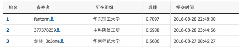 Bowing down to the 0.7 master
Why did I abandon it? As it turns out, this approach did quite well on the "core identification" part, but its fatal flaw was that it depended heavily on segmentation quality. Word segmentation systems often split up long words that make up core entities — for example, "朱家花园" (Zhu Family Garden) gets split into "朱家/花园" (Zhu Family / Garden), and reassembling them afterwards is much harder. So I followed the approach in Chinese Word Segmentation Series #4: seq2seq Character Tagging Based on Bidirectional LSTM, using a word-tagging approach instead, since this approach doesn't heavily depend on segmentation quality. With this approach I eventually reached 0.56 accuracy.
The general steps were:
1. Segment the sentence into words, then train word vectors with Word2Vec;
2. Convert the output into a 5-tag tagging problem: b (first word of a core entity), m (middle of a core entity), e (last word of a core entity), s (single word forming a core entity), x (non-core-entity part);
3. Predict with a two-layer bidirectional LSTM, and use the Viterbi algorithm for tagging.
Finally, it's worth mentioning that this approach could, in principle, be used to do core entity recognition without any word segmentation at all. But overall, segmenting still gives better results, and segmentation also helps reduce sentence length (a 100-character sentence becomes a 50-word sentence after segmentation), which in turn helps reduce the number of model parameters. Here we only need a simple segmentation system, and we don't need its built-in new-word discovery feature.
Transfer Learning
Before actually trying this approach, though, I was quite uncertain about how well it would ultimately perform. The main reason: Baidu provided only 12,000 training samples, but there were 200,000 test samples. With such a lopsided ratio, it seemed hard to expect good results. Moreover, there were 5 tags, and compared to the "x" tag, the other four tags were much rarer — with only 12,000 training samples, there seemed to be a risk of insufficient data.
Of course, practice is the sole criterion for testing truth. This approach hit 0.42 accuracy on its very first test, far higher than the CNN approach I had spent over half a month carefully tuning, so I decided to keep pushing forward with it. Before continuing, I analyzed why this approach worked so well. I think there were two main reasons: one was "transfer learning," and the other was the LSTM's powerful ability to capture semantics.
Traditional data-mining training models are trained purely on the training set. But we can rarely guarantee that the training set matches the test set — more precisely, it's hard to assume that the training set and test set share the same distribution. As a result, even if a model trains extremely well, its test performance can turn out terrible. This isn't caused by overfitting; it's caused by the mismatch between the training and test distributions.
One way to address (or mitigate) this problem is "transfer learning." Transfer learning is by now a fairly comprehensive modeling strategy, so I won't go into detail here. Generally speaking, there are two schemes:
1. Transfer learning before modeling: combine the training set and test set together to learn the features used for modeling, so that the resulting features already incorporate information from the test set;
2. Transfer learning after modeling: if the test-set performance is already decent, say 0.5 accuracy, and you want to improve it further, you can take the test set together with its predicted labels and treat it as additional training data, retraining the model together with the original training samples.
Point 2 might seem confusing — aren't the test-set predictions sometimes wrong? How could feeding in wrong results improve accuracy? Tolstoy said, "Happy families are all alike; every unhappy family is unhappy in its own way." Applied here, I'd put it as: "Correct answers are all alike; wrong answers are each wrong in their own way." That is, if you carry out step 2's training, the correct answers among the test-set predictions will reinforce each other, because they all arise from the same (correct) pattern, whereas the wrong answers each stem from different error patterns. If the model has limited capacity — not enough to overfit — it will tend to smooth out these inconsistent error patterns and gravitate toward the correct answers. Of course, whether this understanding is accurate, I leave to readers to judge. Also, once you get a new round of predictions, you can take only the samples where two consecutive predictions agree as training data, which further raises the proportion of correct answers.
In this competition, transfer learning showed up as follows:
1. Train Word2Vec on the training corpus and test corpus together, so that the word vectors themselves capture the semantics of the test corpus;
2. Train the model on the training corpus;
3. Once the model is obtained, predict on the test corpus, then train a new model using the predictions together with the training corpus;
4. Predict with the new model — performance improves somewhat;
5. Compare the two rounds of predictions: if the two predictions agree, that prediction is likely correct, so use this "likely correct" subset of test results to train the model;
6. Predict with the updated model;
7. If you like, keep repeating steps 4, 5, and 6.
Bidirectional LSTM
The main model architecture:
'''
用最新版本的Keras训练模型,使用GPU加速(我的是GTX 960)
其中Bidirectional函数目前要在github版本才有
'''
from keras.layers import Dense, LSTM, Lambda, TimeDistributed, Input, Masking, Bidirectional
from keras.models import Model
from keras.utils import np_utils
from keras.regularizers import activity_l1 #通过L1正则项,使得输出更加稀疏

sequence = Input(shape=(maxlen, word_size))
mask = Masking(mask_value=0.)(sequence)
blstm = Bidirectional(LSTM(64, return_sequences=True), merge_mode='sum')(mask)
blstm = Bidirectional(LSTM(32, return_sequences=True), merge_mode='sum')(blstm)
output = TimeDistributed(Dense(5, activation='softmax', activity_regularizer=activity_l1(0.01)))(blstm)
model = Model(input=sequence, output=output)
model.compile(loss='categorical_crossentropy', optimizer='adam', metrics=['accuracy'])
This is just a two-layer bidirectional LSTM (I also tried a single layer, but adding an extra layer worked a bit better). The output of each LSTM step is kept, and a softmax is applied at each step — the whole process is basically like a word-segmentation system.
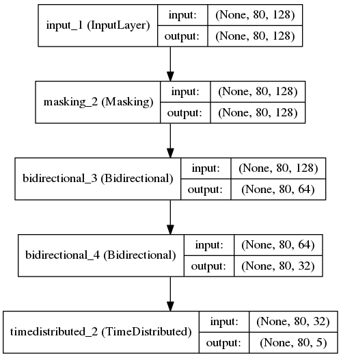 model
model
Of course, how well this model performs also depends heavily on the quality of the word vectors. After a lot of tuning, I found the following word-vector settings to be roughly optimal:
word2vec = gensim.models.Word2Vec(dd['words'].append(d['words']),
                                  min_count=1,
                                  size=word_size,
                                  workers=20,
                                  iter=20,
                                  window=8,
                                  negative=8,
                                  sg=1)
That is, skip-gram works better than CBOW, negative sampling works better than hierarchical softmax, and both the number of negative samples and the window size should be moderate. Of course, this so-called "optimum" is just my own "intuitive impression" after a lot of manual tuning — feel free to run more tests of your own.
About the Competition
I actually noticed this competition, jointly held by Baidu and Xi'an Jiaotong University, last year too, but back then I was still a novice and couldn't handle such a challenging task. This year I gave it a try, and I feel like I gained a lot from it.
First, the competition was organized by Baidu, and that alone makes it appealing, because getting recognition from Baidu generally feels like a big deal, so I was quite looking forward to this kind of competition (hopefully I'll have time to join more of them), and I also hope Baidu keeps running better and better competitions (okay, that's just a polite formality~). Second, through this process I gained a much deeper understanding of language model examples, how to build and use deep networks, and so on — for instance, how CNNs can be applied to language tasks and which language tasks they suit, as well as getting some initial hands-on experience with seq2seq.
Coincidentally, this was an NLP task, while the previous Teddy Cup competition was a computer vision task. Combining the two, I've now worked through the basic tasks in both NLP and computer vision, which gives me a much more solid, grounded feeling about handling these kinds of tasks.
Full Code
Training set link: https://pan.baidu.com/s/1i457nkL Password: stkp
README
Core Entity Recognition Based on Transfer Learning and Bidirectional LSTM
==============================================================
Overall steps (corresponding one-to-one with train_and_predict.py)
==============================================================
1. Segment both the training corpus and the test corpus into words; currently using Jieba segmentation;
2. Convert into a 5-tag tagging problem, constructing the training labels;
3. Train a Word2Vec model on the training corpus and test corpus together;
4. Train a tagging model with a two-layer bidirectional LSTM, based on the seq2seq idea;
5. Predict with the model; prediction accuracy typically fluctuates around 0.46–0.52;
6. Treat the predictions as label data, and retrain the model together with the training data;
7. Predict with the new model; prediction accuracy fluctuates around 0.5–0.55;
8. Compare the two rounds of predictions, take the intersection as label data, and retrain the model together with the training data;
9. Predict with the new model; prediction accuracy stays roughly in the 0.53–0.56 range.
==============================================================
Build environment:
==============================================================
Hardware environment:
1. 96G RAM (in practice, only about 10G was used)
2. GTX960 GPU (for accelerated training)
Software environment:
1. CentOS 7
2. Python 2.7 (all libraries below are third-party Python packages)
3. Jieba segmentation
4. Numpy
5. SciPy
6. Pandas
7. Keras (official GitHub version)
8. Gensim
9. H5PY
10. tqdm
==============================================================
File usage notes:
==============================================================
train_and_predict.py
Contains the entire process from training to prediction. As long as the "unreleased validation data" has the same format as the "released test data" opendata_20w, it can be
placed in the same directory as train_and_predict.py, and then running
python train_and_predict.py
will complete the whole process and generate a series of files:
--------------------------------------------------------------
word2vec_words_final.model, the Word2Vec model
words_seq2seq_final_1.model, the two-layer bidirectional LSTM model obtained the first time
--- result1.txt, the first round of prediction results
--- result1.zip, zip archive of the first round of prediction results
words_seq2seq_final_2.model, the model obtained after the first round of transfer learning
--- result2.txt, the second round of prediction results
--- result2.zip, zip archive of the second round of prediction results
words_seq2seq_final_3.model, the model obtained after the second round of transfer learning
--- result3.txt, the third round of prediction results
--- result3.zip, zip archive of the third round of prediction results
words_seq2seq_final_4.model, the model obtained after the third round of transfer learning
--- result4.txt, the fourth round of prediction results
--- result4.zip, zip archive of the fourth round of prediction results
words_seq2seq_final_5.model, the model obtained after the fourth round of transfer learning
--- result5.txt, the fifth round of prediction results
--- result5.zip, zip archive of the fifth round of prediction results
---------------------------------------------------------------
==============================================================
Approach notes:
==============================================================
Transfer learning is reflected as follows:
1. Train Word2Vec on the training corpus and test corpus together, so that the word vectors themselves capture the semantics of the test corpus;
2. Train the model on the training corpus;
3. Once the model is obtained, predict on the test corpus, then train a new model using the predictions together with the training corpus;
4. Predict with the new model — performance improves somewhat;
5. Compare the two rounds of predictions: if the two predictions agree, that prediction is likely correct, so use this "likely correct" subset of test results to train the model;
6. Predict with the updated model;
7. If you like, keep repeating steps 4, 5, and 6.
The bidirectional LSTM approach:
1. Segmentation;
2. Convert into a 5-tag tagging problem (0: non-core entity, 1: single-word core entity, 2: first word of a multi-word core entity, 3: middle part of a multi-word core entity, 4: last word of a multi-word core entity);
3. Use a bidirectional LSTM to directly output a predicted tag sequence for the input sentence;
4. Use the Viterbi algorithm to obtain the tagging result;
5. Since a regular LSTM has the drawback that later words matter more than earlier ones, a bidirectional LSTM is used instead.
train_and_predict.py (the code hasn't been cleaned up, provided for reference/testing only)
#! -*- coding:utf-8 -*-

'''
基于迁移学习和双向LSTM的核心实体识别

迁移学习体现在:
1、用训练语料和测试语料一起训练Word2Vec,使得词向量本捕捉了测试语料的语义;
2、用训练语料训练模型;
3、得到模型后,对测试语料预测,把预测结果跟训练语料一起训练新的模型;
4、用新的模型预测,模型效果会有一定提升;
5、对比两次预测结果,如果两次预测结果都一样,那说明这个预测结果很有可能是对的,用这部分“很有可能是对的”的测试结果来训练模型;
6、用更新的模型预测;
7、如果你愿意,可以继续重复第4、5、6步。

双向LSTM的思路:
1、分词;
2、转换为5tag标注问题(0:非核心实体,1:单词的核心实体,2:多词核心实体的首词,3:多词核心实体的中间部分,4:多词核心实体的末词);
3、通过双向LSTM,直接对输入句子输出预测标注序列;
4、通过viterbi算法来获得标注结果;
5、因为常规的LSTM存在后面的词比前面的词更重要的弊端,因此用双向LSTM。
'''

import numpy as np
import pandas as pd
import jieba
from tqdm import tqdm
import re

d = pd.read_json('data.json') #训练数据已经被预处理成为标准json格式
d.index = range(len(d)) #重新定义一下索引,当然这只是优化显示效果
word_size = 128 #词向量维度
maxlen = 80 #句子截断长度

'''
修改分词函数,主要是:
1、英文和数字部分不分词,直接返回;
2、双书名号里边的内容不分词;
3、双引号里边如果是十字以内的内容不分词;
4、超出范围内的字符全部替换为空格;
5、分词使用结巴分词,并关闭新词发现功能。
'''

not_cuts = re.compile(u'([\da-zA-Z \.]+)|《(.*?)》|“(.{1,10})”')
re_replace = re.compile(u'[^\u4e00-\u9fa50-9a-zA-Z《》\(\)()“”·\.]')
def mycut(s):
    result = []
    j = 0
    s = re_replace.sub(' ', s)
    for i in not_cuts.finditer(s):
        result.extend(jieba.lcut(s[j:i.start()], HMM=False))
        if s[i.start()] in [u'《', u'“']:
            result.extend([s[i.start()], s[i.start()+1:i.end()-1], s[i.end()-1]])
        else:
            result.append(s[i.start():i.end()])
        j = i.end()
    result.extend(jieba.lcut(s[j:], HMM=False))
    return result

d['words'] = d['content'].apply(mycut) #分词

def label(k): #将输出结果转换为标签序列
    s = d['words'][k]
    r = ['0']*len(s)
    for i in range(len(s)):
        for j in d['core_entity'][k]:
            if s[i] in j:
                r[i] = '1'
                break
    s = ''.join(r)
    r = [0]*len(s)
    for i in re.finditer('1+', s):
        if i.end() - i.start() > 1:
            r[i.start()] = 2
            r[i.end()-1] = 4
            for j in range(i.start()+1, i.end()-1):
                r[j] = 3
        else:
            r[i.start()] = 1
    return r

d['label'] = map(label, tqdm(iter(d.index))) #输出tags

#随机打乱数据
idx = range(len(d))
d.index = idx
np.random.shuffle(idx)
d = d.loc[idx]
d.index = range(len(d))

#读入测试数据并进行分词
dd = open('opendata_20w').read().decode('utf-8').split('\n')
dd = pd.DataFrame([dd]).T
dd.columns = ['content']
dd = dd[:-1]
print u'测试语料分词中......'
dd['words'] = dd['content'].apply(mycut)

'''
用gensim来训练Word2Vec:
1、联合训练语料和测试语料一起训练;
2、经过测试用skip gram效果会好些。
'''
import gensim, logging
logging.basicConfig(format='%(asctime)s : %(levelname)s : %(message)s', level=logging.INFO)

word2vec = gensim.models.Word2Vec(dd['words'].append(d['words']),
                                  min_count=1,
                                  size=word_size,
                                  workers=20,
                                  iter=20,
                                  window=8,
                                  negative=8,
                                  sg=1)
word2vec.save('word2vec_words_final.model')
word2vec.init_sims(replace=True) #预先归一化,使得词向量不受尺度影响

print u'正在进行第一次训练......'

'''
用最新版本的Keras训练模型,使用GPU加速(我的是GTX 960)
其中Bidirectional函数目前要在github版本才有
'''
from keras.layers import Dense, LSTM, Lambda, TimeDistributed, Input, Masking, Bidirectional
from keras.models import Model
from keras.utils import np_utils
from keras.regularizers import activity_l1 #通过L1正则项,使得输出更加稀疏

sequence = Input(shape=(maxlen, word_size))
mask = Masking(mask_value=0.)(sequence)
blstm = Bidirectional(LSTM(64, return_sequences=True), merge_mode='sum')(mask)
blstm = Bidirectional(LSTM(32, return_sequences=True), merge_mode='sum')(blstm)
output = TimeDistributed(Dense(5, activation='softmax', activity_regularizer=activity_l1(0.01)))(blstm)
model = Model(input=sequence, output=output)
model.compile(loss='categorical_crossentropy', optimizer='adam', metrics=['accuracy'])

'''
gen_matrix实现从分词后的list来输出训练样本
gen_target实现将输出序列转换为one hot形式的目标
超过maxlen则截断,不足补0
'''
gen_matrix = lambda z: np.vstack((word2vec[z[:maxlen]], np.zeros((maxlen-len(z[:maxlen]), word_size))))
gen_target = lambda z: np_utils.to_categorical(np.array(z[:maxlen] + [0]*(maxlen-len(z[:maxlen]))), 5)

#从节省内存的角度,通过生成器的方式来训练
def data_generator(data, targets, batch_size):
    idx = np.arange(len(data))
    np.random.shuffle(idx)
    batches = [idx[range(batch_size*i, min(len(data), batch_size*(i+1)))] for i in range(len(data)/batch_size+1)]
    while True:
        for i in batches:
            xx, yy = np.array(map(gen_matrix, data[i])), np.array(map(gen_target, targets[i]))
            yield (xx, yy)

batch_size = 1024
history = model.fit_generator(data_generator(d['words'], d['label'], batch_size), samples_per_epoch=len(d), nb_epoch=200)
model.save_weights('words_seq2seq_final_1.model')

#输出预测结果(原始数据,未整理)
def predict_data(data, batch_size):
    batches = [range(batch_size*i, min(len(data), batch_size*(i+1))) for i in range(len(data)/batch_size+1)]
    p = model.predict(np.array(map(gen_matrix, data[batches[0]])), verbose=1)
    for i in batches[1:]:
        print min(i), 'done.'
        p = np.vstack((p, model.predict(np.array(map(gen_matrix, data[i])), verbose=1)))
    return p

d['predict'] = list(predict_data(d['words'], batch_size))
dd['predict'] = list(predict_data(dd['words'], batch_size))

'''
动态规划部分:
1、zy是转移矩阵,用了对数概率;概率的数值是大概估计的,事实上,这个数值的精确意义不是很大。
2、viterbi是动态规划算法。
'''
zy = {'00':0.15,
      '01':0.15,
      '02':0.7,
      '10':1.0,
      '23':0.5,
      '24':0.5,
      '33':0.5,
      '34':0.5,
      '40':1.0
     }

zy = {i:np.log(zy[i]) for i in zy.keys()}

def viterbi(nodes):
    paths = nodes[0]
    for l in range(1,len(nodes)):
        paths_ = paths.copy()
        paths = {}
        for i in nodes[l].keys():
            nows = {}
            for j in paths_.keys():
                if j[-1]+i in zy.keys():
                    nows[j+i]= paths_[j]+nodes[l][i]+zy[j[-1]+i]
            k = np.argmax(nows.values())
            paths[nows.keys()[k]] = nows.values()[k]
    return paths.keys()[np.argmax(paths.values())]

'''
整理输出结果,即生成提交数据所需要的格式。
整个过程包括:动态规划、结果提取。
'''

def predict(i):
    nodes = [dict(zip(['0','1','2','3','4'], k)) for k in np.log(dd['predict'][i][:len(dd['words'][i])])]
    r = viterbi(nodes)
    result = []
    words = dd['words'][i]
    for j in re.finditer('2.*?4|1', r):
        result.append((''.join(words[j.start():j.end()]), np.mean([nodes[k][r[k]] for k in range(j.start(),j.end())])))
    if result:
        result = pd.DataFrame(result)
        return [result[0][result[1].argmax()]]
    else:
        return result

dd['core_entity'] = map(predict, tqdm(iter(dd.index), desc=u'第一次预测'))

'''
导出提交的JSON格式
'''
gen = lambda i:'[{"content": "'+dd.iloc[i]['content']+'", "core_entity": ["'+''.join(dd.iloc[i]['core_entity'])+'"]}]'
ssss = map(gen, tqdm(range(len(dd))))
result='\n'.join(ssss)
import codecs
f=codecs.open('result1.txt', 'w', encoding='utf-8')
f.write(result)
f.close()
import os
os.system('rm result1.zip')
os.system('zip result1.zip result1.txt')

print u'正在进行第一次迁移学习......'

'''
开始迁移学习。
'''

def label(k): #将输出结果转换为标签序列
    s = dd['words'][k]
    r = ['0']*len(s)
    for i in range(len(s)):
        for j in dd['core_entity'][k]:
            if s[i] in j:
                r[i] = '1'
                break
    s = ''.join(r)
    r = [0]*len(s)
    for i in re.finditer('1+', s):
        if i.end() - i.start() > 1:
            r[i.start()] = 2
            r[i.end()-1] = 4
            for j in range(i.start()+1, i.end()-1):
                r[j] = 3
        else:
            r[i.start()] = 1
    return r

dd['label'] = map(label, tqdm(iter(dd.index))) #输出tags

'''
将测试集和训练集一起放到模型中训练,
其中测试集的样本权重设置为1,训练集为10
'''
w = np.array([1]*len(dd) + [10]*len(d))
def data_generator(data, targets, batch_size):
    idx = np.arange(len(data))
    np.random.shuffle(idx)
    batches = [idx[range(batch_size*i, min(len(data), batch_size*(i+1)))] for i in range(len(data)/batch_size+1)]
    while True:
        for i in batches:
            xx, yy = np.array(map(gen_matrix, data[i])), np.array(map(gen_target, targets[i]))
            yield (xx, yy, w[i])

history = model.fit_generator(data_generator(
                                    dd[['words']].append(d[['words']], ignore_index=True)['words'],
                                    dd[['label']].append(d[['label']], ignore_index=True)['label'],
                                    batch_size),
                              samples_per_epoch=len(dd)+len(d),
                              nb_epoch=20)

model.save_weights('words_seq2seq_final_2.model')
d['predict'] = list(predict_data(d['words'], batch_size))
dd['predict'] = list(predict_data(dd['words'], batch_size))
dd['core_entity_2'] = map(predict, tqdm(iter(dd.index), desc=u'第一次迁移学习预测'))

'''
导出提交的JSON格式
'''
gen = lambda i:'[{"content": "'+dd.iloc[i]['content']+'", "core_entity": ["'+''.join(dd.iloc[i]['core_entity_2'])+'"]}]'
ssss = map(gen, tqdm(range(len(dd))))
result='\n'.join(ssss)
import codecs
f=codecs.open('result2.txt', 'w', encoding='utf-8')
f.write(result)
f.close()
import os
os.system('rm result2.zip')
os.system('zip result2.zip result2.txt')

print u'正在进行第二次迁移学习......'

'''
开始迁移学习2。
'''

ddd = dd[dd['core_entity'] == dd['core_entity_2']].copy()

'''
将测试集和训练集一起放到模型中训练,
其中测试集的样本权重设置为1,训练集为5
'''
w = np.array([1]*len(ddd) + [5]*len(d))
def data_generator(data, targets, batch_size):
    idx = np.arange(len(data))
    np.random.shuffle(idx)
    batches = [idx[range(batch_size*i, min(len(data), batch_size*(i+1)))] for i in range(len(data)/batch_size+1)]
    while True:
        for i in batches:
            xx, yy = np.array(map(gen_matrix, data[i])), np.array(map(gen_target, targets[i]))
            yield (xx, yy, w[i])

history = model.fit_generator(data_generator(
                                    ddd[['words']].append(d[['words']], ignore_index=True)['words'],
                                    ddd[['label']].append(d[['label']], ignore_index=True)['label'],
                                    batch_size),
                              samples_per_epoch=len(ddd)+len(d),
                              nb_epoch=20)

model.save_weights('words_seq2seq_final_3.model')
d['predict'] = list(predict_data(d['words'], batch_size))
dd['predict'] = list(predict_data(dd['words'], batch_size))
dd['core_entity_3'] = map(predict, tqdm(iter(dd.index), desc=u'第二次迁移学习预测'))

'''
导出提交的JSON格式
'''
gen = lambda i:'[{"content": "'+dd.iloc[i]['content']+'", "core_entity": ["'+''.join(dd.iloc[i]['core_entity_3'])+'"]}]'
ssss = map(gen, tqdm(range(len(dd))))
result='\n'.join(ssss)
import codecs
f=codecs.open('result3.txt', 'w', encoding='utf-8')
f.write(result)
f.close()
import os
os.system('rm result3.zip')
os.system('zip result3.zip result3.txt')

print u'正在进行第三次迁移学习......'

'''
开始迁移学习3。
'''

ddd = dd[dd['core_entity'] == dd['core_entity_2']].copy()
ddd = ddd[ddd['core_entity_3'] == ddd['core_entity_2']].copy()

'''
将测试集和训练集一起放到模型中训练,
其中测试集的样本权重设置为1,训练集为1
'''
w = np.array([1]*len(ddd) + [1]*len(d))
def data_generator(data, targets, batch_size):
    idx = np.arange(len(data))
    np.random.shuffle(idx)
    batches = [idx[range(batch_size*i, min(len(data), batch_size*(i+1)))] for i in range(len(data)/batch_size+1)]
    while True:
        for i in batches:
            xx, yy = np.array(map(gen_matrix, data[i])), np.array(map(gen_target, targets[i]))
            yield (xx, yy, w[i])

history = model.fit_generator(data_generator(
                                    ddd[['words']].append(d[['words']], ignore_index=True)['words'],
                                    ddd[['label']].append(d[['label']], ignore_index=True)['label'],
                                    batch_size),
                              samples_per_epoch=len(ddd)+len(d),
                              nb_epoch=20)

model.save_weights('words_seq2seq_final_4.model')
d['predict'] = list(predict_data(d['words'], batch_size))
dd['predict'] = list(predict_data(dd['words'], batch_size))
dd['core_entity_4'] = map(predict, tqdm(iter(dd.index), desc=u'第三次迁移学习预测'))

'''
导出提交的JSON格式
'''
gen = lambda i:'[{"content": "'+dd.iloc[i]['content']+'", "core_entity": ["'+''.join(dd.iloc[i]['core_entity_4'])+'"]}]'
ssss = map(gen, tqdm(range(len(dd))))
result='\n'.join(ssss)
import codecs
f=codecs.open('result4.txt', 'w', encoding='utf-8')
f.write(result)
f.close()
import os
os.system('rm result4.zip')
os.system('zip result4.zip result4.txt')

print u'正在进行第四次迁移学习......'

'''
开始迁移学习4。
'''

ddd = dd[dd['core_entity'] == dd['core_entity_2']].copy()
ddd = ddd[ddd['core_entity_3'] == ddd['core_entity_2']].copy()
ddd = ddd[ddd['core_entity_4'] == ddd['core_entity_2']].copy()

'''
将测试集和训练集一起放到模型中训练,
其中测试集的样本权重设置为1,训练集为1
'''
w = np.array([1]*len(ddd) + [1]*len(d))
def data_generator(data, targets, batch_size):
    idx = np.arange(len(data))
    np.random.shuffle(idx)
    batches = [idx[range(batch_size*i, min(len(data), batch_size*(i+1)))] for i in range(len(data)/batch_size+1)]
    while True:
        for i in batches:
            xx, yy = np.array(map(gen_matrix, data[i])), np.array(map(gen_target, targets[i]))
            yield (xx, yy, w[i])

history = model.fit_generator(data_generator(
                                    ddd[['words']].append(d[['words']], ignore_index=True)['words'],
                                    ddd[['label']].append(d[['label']], ignore_index=True)['label'],
                                    batch_size),
                              samples_per_epoch=len(ddd)+len(d),
                              nb_epoch=20)

model.save_weights('words_seq2seq_final_5.model')
d['predict'] = list(predict_data(d['words'], batch_size))
dd['predict'] = list(predict_data(dd['words'], batch_size))
dd['core_entity_5'] = map(predict, tqdm(iter(dd.index), desc=u'第四次迁移学习预测'))

'''
导出提交的JSON格式
'''
gen = lambda i:'[{"content": "'+dd.iloc[i]['content']+'", "core_entity": ["'+''.join(dd.iloc[i]['core_entity_5'])+'"]}]'
ssss = map(gen, tqdm(range(len(dd))))
result='\n'.join(ssss)
import codecs
f=codecs.open('result5.txt', 'w', encoding='utf-8')
f.write(result)
f.close()
import os
os.system('rm result5.zip')
os.system('zip result5.zip result5.txt')
Translated automatically with claude-sonnet-5; all equations are reproduced verbatim from the source. Copyright remains with the original author.