[Chinese Word Segmentation Series] 4. Sequence-to-Sequence Character Tagging Based on Bidirectional LSTM
On the Character-Tagging Approach
The previous post discussed the character-tagging approach to word segmentation. It's worth noting that character tagging is a genuinely powerful method — otherwise it wouldn't have achieved top results in public benchmarks. In my view, there are two main reasons why character tagging works so well. The first is that it turns word segmentation into a sequence-labeling problem, and one where the labeling is aligned — that is, each input character corresponds one-to-one with an output label, which is a fairly mature setup within sequence labeling. The second reason is that this tagging scheme is, in effect, already a process of summarizing semantic regularities. Take the 4-tag scheme as an example: we know that the character "李" (Li) is a common surname, and about half the time it appears as the first character of a multi-character word (like a name), so it's often tagged b; meanwhile "想" (xiang), due to words like "理想" (ideal), is often tagged e. As a result, when "李想" appears together, even if "李想" never appeared in the vocabulary before, the model can still correctly output be — recognizing "李想" as a single word (in this case, a person's name). It's precisely for this reason that even the HMM model, often regarded as the least accurate approach, can still perform reasonably well.
There's another point worth discussing regarding tagging: the number of tags. The commonly used scheme is 4-tag, though 6-tag and 2-tag schemes also exist. The simplest way to mark segmentation results would seem to be 2-tag — just marking "split" versus "no split" — but this doesn't work well in practice. Why does using more tags actually give better results? Because a larger tag set captures semantic regularities more comprehensively. For instance, with 4-tag labeling we can learn which characters commonly appear alone as single-character words, which characters tend to start a word, and which tend to end one. With only 2-tag labeling, we can only learn which characters tend to start a word — which, from an inductive standpoint, is far less complete. But how does 6-tag compare to 4-tag? I don't think it's necessarily better. 6-tag requires additionally learning which characters tend to appear as the second or third character of a word — but is this really a meaningful angle to summarize? It seems to me there aren't really characters that are reliably tied to being the second or third character; this kind of regularity is much weaker than the regularities around first and last characters. (That said, from the perspective of new-word discovery, 6-tag does make it easier to detect longer words.)
Bidirectional LSTM
The way to understand bidirectional LSTM is this: bidirectional LSTM is an improved version of LSTM, and LSTM is an improved version of RNN. So, we first need to understand RNN.
I once mentioned in my earlier piece From Boosting to Neural Networks: Is a Mountain Still a Mountain? that a model's output is, in fact, itself a kind of feature, and can be fed back in as input to the model — and this is exactly the kind of network structure RNNs embody. An ordinary multilayer neural network is a one-way propagation process from input to output. This can also be applied to high-dimensional inputs, but with too many nodes, training becomes hard, and overfitting becomes a risk. For example, a 1000x1000 image input is difficult to handle directly — this is what motivated CNNs. Or take a 1000-word sentence, with each word represented as a 100-dimensional word embedding — the input dimensionality is still quite large. One solution here is RNN (CNN can also be used, but RNN is better suited to sequence problems).
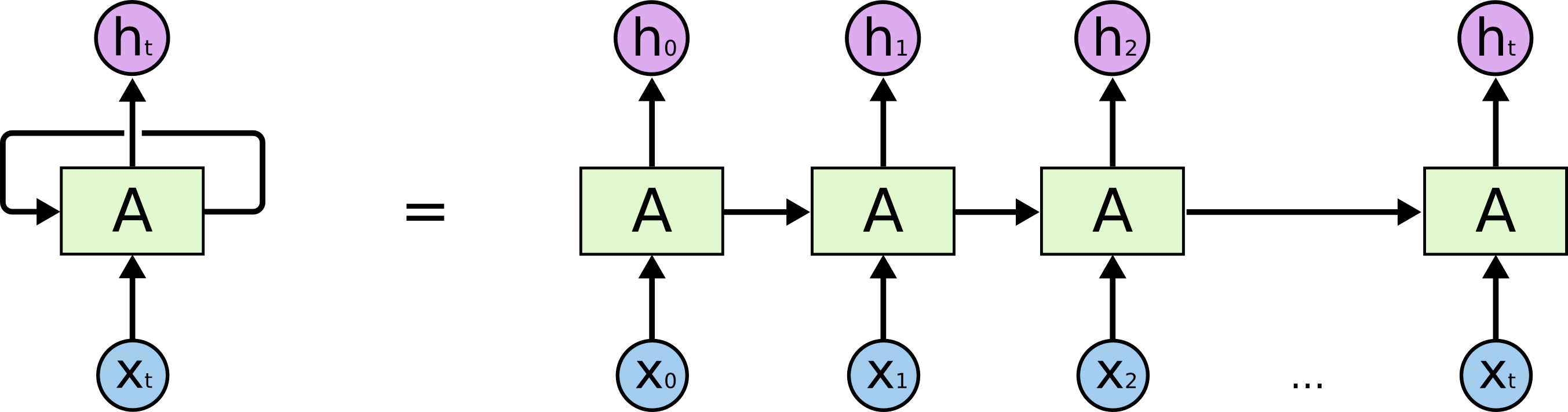 The RNN process
What RNN does is this: to predict the final result, I first make a prediction using the first word. Of course, relying solely on the first word's prediction won't be very accurate, so I take that result as a feature, and combine it with the second word to make a prediction; then I take this new prediction result and combine it with the third word to make a further new prediction; and I repeat this process all the way to the last word. So, if the input has n words, we actually make n predictions on the result, yielding n predicted sequences. Throughout this process, the model shares a single set of parameters. As a result, RNN reduces the number of parameters in the model, which helps prevent overfitting, and since it was designed from the ground up to handle sequential problems, it's particularly well suited to them.
LSTM improves on RNN, enabling it to capture longer-range dependencies. But whether LSTM or RNN, there is a shared issue: information flows from left to right, so later words end up carrying more weight than earlier ones. This is problematic for the segmentation task, since every character in a sentence should be treated with equal importance. This is why bidirectional LSTM was introduced: it runs an LSTM pass from left to right, then another from right to left, and combines the two results.
Application to the Word Segmentation Task
People have experimented with deep learning for word segmentation for quite a while now — see, for example, the following articles:
http://blog.csdn.net/itplus/article/details/13616045
https://github.com/xccds/chinese_wordseg_keras
http://www.leiphone.com/news/201608/IWvc75oJglAIsDvJ.html
In these articles, whether using a simple neural network or LSTM, the approach is essentially the same as in traditional models: the label of the current character is predicted from its context, where the context is a fixed window — for instance, using the 5 characters before and after, plus the current character, to predict its label. There's nothing wrong with this approach per se, but it merely swaps out the traditional probability-estimation methods — HMM, Maximum Entropy, CRF, etc. — for a neural network, while keeping the overall framework unchanged. Fundamentally, it's still an n-gram model. But with LSTM, since it can inherently produce sequence-to-sequence (seq2seq) output, why not directly output the label sequence for the entire original sentence? Wouldn't that actually make full use of the whole-sentence information? That's exactly what this post attempts.
An LSTM can produce an output sequence from an input sequence, and this output sequence takes contextual relationships into account. So we can attach a softmax classifier to each position in the output sequence to predict the probability of each label. Based on this sequence-to-sequence idea, we can directly predict the label sequence for a whole sentence.
Keras Implementation
No time to waste — let's get to it. The word embedding dimension used is 128, and sentences are truncated to a length of 32 (samples longer than 32 characters are discarded — there are very few of these, since after splitting on natural delimiters like commas and periods, sentences rarely exceed 32 characters). This time I used 5 tags: on top of the original 4-tag scheme, I added an x tag to mark the padded portion for sentences shorter than 32 characters — for example, if a sentence has 20 characters, then positions 21 through 32 are all labeled x.
For data, I used the portion of the Bakeoff 2005 corpus provided by Microsoft Research. The code is below — feel free to leave a comment if anything is unclear.
# -*- coding:utf-8 -*-
import re
import numpy as np
import pandas as pd

s = open('msr_train.txt').read().decode('gbk')
s = s.split('\r\n')

def clean(s): #整理一下数据,有些不规范的地方
    if u'“/s' not in s:
        return s.replace(u' ”/s', '')
    elif u'”/s' not in s:
        return s.replace(u'“/s ', '')
    elif u'‘/s' not in s:
        return s.replace(u' ’/s', '')
    elif u'’/s' not in s:
        return s.replace(u'‘/s ', '')
    else:
        return s

s = u''.join(map(clean, s))
s = re.split(u'[,。!?、]/[bems]', s)

data = [] #生成训练样本
label = []
def get_xy(s):
    s = re.findall('(.)/(.)', s)
    if s:
        s = np.array(s)
        return list(s[:,0]), list(s[:,1])

for i in s:
    x = get_xy(i)
    if x:
        data.append(x[0])
        label.append(x[1])

d = pd.DataFrame(index=range(len(data)))
d['data'] = data
d['label'] = label
d = d[d['data'].apply(len) <= maxlen]
d.index = range(len(d))
tag = pd.Series({'s':0, 'b':1, 'm':2, 'e':3, 'x':4})

chars = [] #统计所有字,跟每个字编号
for i in data:
    chars.extend(i)

chars = pd.Series(chars).value_counts()
chars[:] = range(1, len(chars)+1)

#生成适合模型输入的格式
from keras.utils import np_utils
d['x'] = d['data'].apply(lambda x: np.array(list(chars[x])+[0]*(maxlen-len(x))))

def trans_one(x):
    _ = map(lambda y: np_utils.to_categorical(y,5), tag[x].reshape((-1,1)))
    _ = list(_)
    _.extend([np.array([[0,0,0,0,1]])]*(maxlen-len(x)))
    return np.array(_)

d['y'] = d['label'].apply(trans_one)

#设计模型
word_size = 128
maxlen = 32
from keras.layers import Dense, Embedding, LSTM, TimeDistributed, Input, Bidirectional
from keras.models import Model

sequence = Input(shape=(maxlen,), dtype='int32')
embedded = Embedding(len(chars)+1, word_size, input_length=maxlen, mask_zero=True)(sequence)
blstm = Bidirectional(LSTM(64, return_sequences=True), merge_mode='sum')(embedded)
output = TimeDistributed(Dense(5, activation='softmax'))(blstm)
model = Model(input=sequence, output=output)
model.compile(loss='categorical_crossentropy', optimizer='adam', metrics=['accuracy'])

batch_size = 1024
history = model.fit(np.array(list(d['x'])), np.array(list(d['y'])).reshape((-1,maxlen,5)), batch_size=batch_size, nb_epoch=50)

#转移概率,单纯用了等概率
zy = {'be':0.5,
      'bm':0.5,
      'eb':0.5,
      'es':0.5,
      'me':0.5,
      'mm':0.5,
      'sb':0.5,
      'ss':0.5
     }

zy = {i:np.log(zy[i]) for i in zy.keys()}

def viterbi(nodes):
    paths = {'b':nodes[0]['b'], 's':nodes[0]['s']}
    for l in range(1,len(nodes)):
        paths_ = paths.copy()
        paths = {}
        for i in nodes[l].keys():
            nows = {}
            for j in paths_.keys():
                if j[-1]+i in zy.keys():
                    nows[j+i]= paths_[j]+nodes[l][i]+zy[j[-1]+i]
            k = np.argmax(nows.values())
            paths[nows.keys()[k]] = nows.values()[k]
    return paths.keys()[np.argmax(paths.values())]

def simple_cut(s):
    if s:
        r = model.predict(np.array([list(chars[list(s)].fillna(0).astype(int))+[0]*(maxlen-len(s))]), verbose=False)[0][:len(s)]
        r = np.log(r)
        nodes = [dict(zip(['s','b','m','e'], i[:4])) for i in r]
        t = viterbi(nodes)
        words = []
        for i in range(len(s)):
            if t[i] in ['s', 'b']:
                words.append(s[i])
            else:
                words[-1] += s[i]
        return words
    else:
        return []

not_cuts = re.compile(u'([\da-zA-Z ]+)|[。,、?!\.\?,!]')
def cut_word(s):
    result = []
    j = 0
    for i in not_cuts.finditer(s):
        result.extend(simple_cut(s[j:i.start()]))
        result.append(s[i.start():i.end()])
        j = i.end()
    result.extend(simple_cut(s[j:]))
    return result
We can inspect the model's structure using model.summary().
model.summary()
_______________________________________________________
Layer (type) Output Shape Param # Connected to
=======================================================
input_2 (InputLayer) (None, 32) 0
_______________________________________________________
embedding_2 (Embedding) (None, 32, 128) 660864 input_2[0][0]
_______________________________________________________
bidirectional_1 (Bidirectional) (None, 32, 64) 98816 embedding_2[0][0]
_______________________________________________________
timedistributed_2 (TimeDistribute) (None, 32, 5) 325 bidirectional_1[0][0]
=======================================================
Total params: 760005
_______________________________________________________
How does the final model perform? I won't bother comparing it against the usual benchmark scores — getting over 90% accuracy on the test set isn't difficult with a model like this these days. What I really care about is how it handles new-word recognition and ambiguity resolution. Below are some test results (chosen somewhat arbitrarily):
RNN 的 意思 是 , 为了 预测 最后 的 结果 , 我 先 用 第一个 词 预测 , 当然 , 只 用 第一个 预测 的 预测 结果 肯定 不 精确 , 我 把 这个 结果 作为 特征 , 跟 第二词 一起 , 来 预测 结果 ; 接着 , 我 用 这个 新 的 预测 结果 结合 第三词 , 来 作 新 的 预测 ; 然后 重复 这个 过程 。
结婚 的 和 尚未 结婚 的
苏剑林 是 科学 空间 的 博主 。
广东省 云浮市 新兴县
魏则西 是 一 名 大学生
这 真是 不堪入目 的 环境
列夫·托尔斯泰 是 俄罗斯 一 位 著名 的 作家
保加利亚 首都 索非亚 是 全国 政治 、 经济 、 文化中心 , 位于 保加利亚 中 西部
罗斯福 是 第二次世界大战 期间 同 盟国 阵营 的 重要 领导人 之一 。 1941 年 珍珠港 事件发生 后 , 罗斯 福力 主对 日本 宣战 , 并 引进 了 价格 管制 和 配给 。 罗斯福 以 租 借 法案 使 美国 转变 为 “ 民主 国家 的 兵工厂 ” , 使 美国 成为 同 盟国 主要 的 军火 供应商 和 融资 者 , 也 使得 美国 国内 产业 大幅 扩张 , 实现 充分 就业 。 二战 后期 同 盟国 逐渐 扭转 形势 后 , 罗斯福 对 塑造 战后 世界 秩序 发挥 了 关键 作用 , 其 影响 力 在 雅尔塔 会议 及 联合国 的 成立 中 尤其 明显 。 后来 , 在 美国 协助 下 , 盟军 击败 德国 、 意大利 和 日本 。
As you can see, the results are quite encouraging. Whether it's Chinese or foreign personal names, or place names, the recognition performance is good. That's all I'll say about this model for now — I'll keep digging into it further down the line.
Final Remarks
This post essentially provides a framework for directly tagging a sequence using bidirectional LSTM, producing a complete tag sequence. This tagging approach can be applied to many tasks, such as part-of-speech tagging and entity recognition. So the idea of seq2seq tagging based on bidirectional LSTM has quite broad applicability and is well worth further study. Even the currently popular neural machine translation models are, in fact, built on this same sequence-to-sequence paradigm.
Translated automatically with claude-sonnet-5; all equations are reproduced verbatim from the source. Copyright remains with the original author.