From Boosting to Neural Networks: Mountains as Mountains?

从Boosting学习到神经网络：看山是山？ 苏剑林 · 2016-07-01 · Machine Learning neural network boosting sentiment classification

A while back, in Chaozhou, in between lecturing Han Shi's students on text mining, I found myself dipping into Boosting algorithms and doing a bit of brainstorming about them. In the end, I managed to sort out some of the essential features of Boosting, and along the way stumbled onto an unexpected result: some of the theoretical proofs behind the AdaBoost algorithm can also be used to explain why neural network models are so powerful.

The AdaBoost Algorithm

Boosting belongs to the family of ensemble methods, though really it's less an algorithm than a way of thinking about problem-solving. Take a supervised classification problem as an example: the idea is that if you combine a bunch of weak classifiers (each only needing accuracy strictly better than random) in the right way, you can end up with an excellent classifier — one that, in theory, can reach 100% accuracy. AdaBoost is one concrete instance of a Boosting algorithm, proposed by Schapire in 1996; it lays out a specific scheme for Boosting learning and gives a theoretical proof about the error rate.

Let's take a binary classification problem as an example. Suppose we have a batch of samples $\{x_i,y_i\},i=1,2,\dots,n$, where $x_i$ is the sample data (possibly multi-dimensional input) and $y_i\in\{1,-1\}$ is the label. Here we use 1 and -1 to describe the labels rather than the usual 1 and 0, purely for convenience in the proof later — there's nothing special about it. Next, suppose we already have a weak classifier $G(x)$ — logistic regression, an SVM, a decision tree, whatever — the only requirement being that its accuracy is strictly better than random (i.e., strictly greater than 0.5 for a binary problem). "Strictly better" means there exists some constant $\epsilon$ greater than 0 such that the accuracy is always at least $\frac{1}{2}+\epsilon$. (more)

The idea behind AdaBoost is: each time before training the weak classifier $G(x)$, assign different weights $w_{k,1},w_{k,2},\dots,w_{k,n}$ to the samples (raising the weight of samples that were previously misclassified). This way, each round produces a different model with different parameters $G_1(x),G_2(x),\dots,G_m(x)$ (which could either be different parameterizations of the same model, or an ensemble of different models altogether). These are then combined as follows:

$$y=\bar{G}(x)=\text{sign}[f(x)]=\text{sign}\left[\sum_{k=1}^m \alpha_k G_k(x)\right]$$

Here $f(x)=\sum_{k=1}^m \alpha_k G_k(x)$, and it can ultimately be proven that the classifier $\bar{G}(x)$ obtained this way performs excellently. Since AdaBoost itself isn't the main focus of this post, to avoid getting sidetracked I've put the detailed mathematical derivation at the end.

Mountains as Mountains, Rivers as Rivers

Setting aside the mathematical details, let's think about what AdaBoost is actually doing. Or, to ask a broader question, what is the essence of an ensemble model?

When building a classification model, the usual process looks like this:

1. Gather a batch of labeled data — say, sentiment-labeled reviews for a text sentiment classification model;
2. Construct features;
3. Choose an appropriate model — logistic regression, SVM, neural network, etc.;
4. Feed the data into the model and train it;
5. Examine the results and iterate.

Beginners often pour their energy into step 3, becoming enamored with highly nonlinear, high-precision models. In reality, though, models with high precision usually owe their strength to a fairly powerful feature-construction process upstream. If the features are well built, even a simple linear model (like logistic regression) can achieve high accuracy. In other words, the most important step in modeling should really be step 2 — feature construction.

Of course, constructing good features is also the hardest part. Doing it well requires a thorough understanding of the data, and sometimes fairly specialized domain knowledge. There's no unified method for combining existing features into better ones. At this stage, we tend to agonize over feature construction and hope for a pleasant surprise in the prediction results. This is what we might call "seeing mountains as mountains, rivers as rivers" (seeing features as features, results as results).

Mountains Are Not Mountains, Rivers Are Not Rivers

But why not think a bit more wildly? Suppose again we have a binary classification task — text sentiment classification, say. We train a model, such as logistic regression, on the available data, obtain its parameters, and get some prediction results with accuracy above 50%. Are these results really just results?

Mathematically speaking, this result comes from a linear combination of the original data, followed by a nonlinear transformation via a logistic function — in plain terms, it's something derived from the original features through some operation. Given that, why not regard it as itself a way of constructing a feature?

Exactly — it's a result, but it's also a feature! You use one set of weights to train a logistic regression model and get a batch of predictions; you use a different set of weights to train another logistic regression model with different parameters and get another batch of predictions; and so on. Why not treat this batch of results as features and feed them into yet another logistic regression model? At worst, this new model won't be any less accurate than the original single model, right? And so we arrive at a rather remarkable conclusion — a model can be used both to produce results and to construct features: the result is the feature. This is the point at which we reach "mountains are not mountains, rivers are not rivers" — the boundary between features and results has dissolved.

At this point, things may suddenly click — the essence of Boosting is really nothing more than treating a model's output as a feature, and then modeling again on top of it. Since a model's outputs are generally already decent features, this last step can substantially boost the classifier's performance — good features naturally lead to good accuracy.

At this point, I really do want to quote Laozi: "The Tao that can be spoken is not the eternal Tao; the name that can be named is not the eternal name."

Mountains Are Again Mountains, Rivers Are Again Rivers

This is a new perspective — treating a model's output as a constructed feature. But have we really never used this trick before?

As it turns out, we have, just perhaps not so explicitly. Suppose we have a binary classification problem (say, predicting whether someone smokes), and one of the features is gender, taking values male/female. How do we quantify this to feed into the model? We might use 1 for male and 0 for female. But isn't this equivalent to constructing the following model?

$$G(x)=\left\{\begin{aligned}&1,\quad x=\text{male}\\ &0,\quad x=\text{female}\end{aligned}\right.$$

Clearly, this can be seen as a model in its own right (its input being gender, its output being whether the person smokes, with 1 meaning "smokes") used to predict whether an individual smokes. What was originally just a way of representing a feature has now become the prediction output of a model — and then we feed that model's output into a new model for further prediction. Looking back at this process, isn't this again a matter of treating a result as a feature to be fed into a model?

It turns out we've been using this idea for a long time, just not so overtly. Coming back to it now, we realize this way of thinking shows up all over data mining — perhaps we've come full circle and arrived at "mountains are again mountains, rivers are again rivers." The Boosting algorithm (AdaBoost) can be seen as taking this idea and running with it. And once we look at the description of neural networks below, this feeling becomes even stronger.

Neural Networks

Yet the model that truly pushes this idea to its logical extreme is the neural network.

Does the neural network model really have something to do with Boosting? Indeed it does — a neural network can be viewed as a special, strengthened case of AdaBoost, and this lets us borrow AdaBoost's theoretical proofs to explain why neural networks are so powerful.

What do I mean by this? Let's revisit the passage from earlier:

Exactly — it's a result, but it's also a feature! You use one set of weights to train a logistic regression model and get a batch of predictions; you use a different set of weights to train another logistic regression model with different parameters and get another batch of predictions; and so on. Why not treat this batch of results as features and feed them into yet another logistic regression model? At worst, this new model won't be any less accurate than the original single model, right?

What does this process look like when drawn as a diagram? See below.

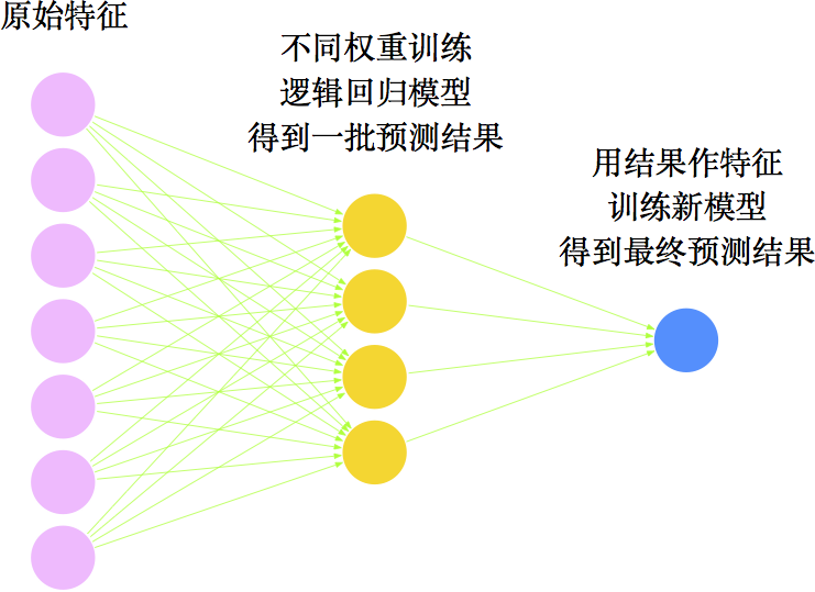AdaBoost learning process

At first glance, isn't this exactly a three-layer network model?

Indeed it is — this is precisely a three-layer neural network! Choose logistic regression as the weak classifier, combine it via the AdaBoost algorithm, and the result is equivalent to a three-layer neural network model! That said, neural networks are actually a bit smarter about it. AdaBoost trains step by step, much like a greedy algorithm, and so is quite likely to land only on a locally optimal solution. Neural networks, in contrast, leave all parameters undetermined and optimize them jointly using a single loss function; as long as the optimization algorithm is good enough, it can find the optimal solution. From this angle, neural networks have the edge. Moreover, neural networks can stack even more layers on top of this (which can also be viewed as using AdaBoost itself as a weak classifier and composing it repeatedly to get an even better classifier), improving performance further. This is one reason why, in today's era of deep learning, the practical significance of AdaBoost has diminished — though its core idea remains deeply insightful.

Not only that, but from this same angle — "treat the prediction result as a feature" — we can even arrive at the structure of the RNN (recurrent neural network)! Notice that in the current AdaBoost algorithm, the final model-building step only uses the outputs of previous models as features. Why not use both the previous outputs and the original raw data together as features for the model? If we actually did this, we'd end up with a prototype of the RNN — feeding the previous output back in as part of the current input.

At this point, the neural network becomes a special case of AdaBoost, but at the same time also a strengthened version of it. Perhaps we could say that the neural network has pushed the idea of ensemble modeling to its absolute limit.

At this point, one could say Boosting is everywhere — truly "mountains are again mountains, rivers are again rivers." Because Boosting has never really been just a standalone model; it's a profound way of thinking about problem-solving — and profound ideas tend to leave a lasting mark.

Appendix: Derivation of the AdaBoost Algorithm

AdaBoost itself isn't hard to understand, but the real question is how to choose the various $w$ and $\alpha$. Schapire proposed a scheme for this:

1. Initialize $w_{1,1}=w_{1,2}=\dots=w_{1,n}=\frac{1}{n}$ at the start, and use these as weights to train a classifier $G_1(x)$;
2. At each subsequent step, update $w$ and $\alpha$ as follows:
$$\begin{aligned}&\alpha_k=\frac{1}{2}\log\frac{1-\varepsilon_k}{\varepsilon_k}\\ > &w_{k+1,i}=\frac{1}{Z_k}w_{k,i}\exp\left(-\alpha_k y_i G_k(x_i)\right)\end{aligned}$$

Here $\varepsilon_k$ is the error rate — that is, using the model $G_k(x)$ to make predictions, the number of misclassified samples divided by $n$. Written as a formula:

$$\varepsilon_k = \sum_{i=1}^n w_{k,i} I\left(-y_i G_k(x_i)\right)$$

Here $I(x)$ is the indicator function that counts positives:

$$I(x)=\left\{\begin{aligned}&1,\quad x > 0\\ &0,\quad x\leq 0\end{aligned}\right.$$

When the prediction is correct, $-y_i G_k(x_i)=-1$, so $I\left(-y_i G_k(x_i)\right)=0$; otherwise $I\left(-y_i G_k(x_i)\right)=1$, so $\sum_{i=1}^n I\left(-y_i G_k(x_i)\right)$ simply counts the number of mistakes. And $Z_k=\sum_{i=1}^n w_{k,i}\exp\left(-\alpha_k y_i G_k(x_i)\right)$ is a normalization factor.

The biggest question, of course, is why choose things this way? I don't know exactly how Schapire arrived at it either, but perhaps we can find some hints by analyzing the error rate. The error rate of the final classifier $\bar{G}(x)$ can be estimated as

$$\begin{aligned}\varepsilon &= \frac{1}{n} \sum_{i=1}^{n} I\left(-y_i \bar{G}(x_i)\right) \\ &= \frac{1}{n} \sum_{i=1}^{n} I\left(-y_i f(x_i)\right) \\ & < \frac{1}{n} \sum_{i=1}^{n} \exp\left(-y_i f(x_i)\right) \end{aligned}$$

where we've used $I(x)\leq\max(0,1+x) < \max(0,e^x)=e^x$. At this point, we can substitute in the expression for $f$:

$$\begin{aligned}&\frac{1}{n} \sum_{i=1}^{n} \exp(-y_i f(x_i))\\ =&\frac{1}{n}\sum_{i=1}^{n} \exp\left(-y_i \sum_{k=1}^m \alpha_k G_k (x)\right)\\ =&\frac{1}{n}\sum_{i=1}^{n} \prod_{k=1}^m\exp\left(-y_i \alpha_k G_k (x)\right)\\ =&\sum_{i=1}^{n} w_{1,i}\prod_{k=1}^m\exp\left(-y_i \alpha_k G_k (x)\right)\\ =&\sum_{i=1}^{n} w_{1,i}\exp\left(-y_i \alpha_1 G_1 (x)\right)\prod_{k=2}^m\exp\left(-y_i \alpha_k G_k (x)\right)\\ =&Z_1\sum_{i=1}^{n} w_{2,i}\prod_{k=2}^m\exp\left(-y_i \alpha_k G_k (x)\right)\\ =&\dots\\ =&Z_1 Z_2 \dots Z_m \end{aligned}$$

Recalling the expression for $Z_k$:

$$Z_k=\sum_{i=1}^n w_{k,i}\exp\left(-\alpha_k y_i G_k(x_i)\right)$$

Note that although the term $\exp\left(-\alpha_k y_i G_k(x_i)\right)$ looks complicated, in fact it can only take one of two values — $e^{-\alpha_k}$, indicating a correct prediction, or $e^{\alpha_k}$, indicating a misclassification. Therefore:

$$\begin{aligned}Z_k=&\sum_{i=1}^n w_{k,i}\exp\left(-\alpha_k y_i G_k(x_i)\right)\\ =&\sum_{\text{correct prediction}} w_{k,i}e^{-\alpha_k}+\sum_{\text{wrong prediction}} w_{k,i}e^{\alpha_k}\\ =&e^{-\alpha_k}\sum_{\text{correct prediction}} w_{k,i}+e^{\alpha_k}\sum_{\text{wrong prediction}} w_{k,i}\\ =&e^{-\alpha_k}(1-\varepsilon_k)+e^{\alpha_k} \varepsilon_k\\ = &2\sqrt{(1-\varepsilon_k)\varepsilon_k} \quad(\text{substitute}\alpha_k=\frac{1}{2}\log\frac{1-\varepsilon_k}{\varepsilon_k}\text{thus})\\ =&\sqrt{1-4\gamma_k^2}\quad (\text{denote}\gamma_k = \frac{1}{2}-\varepsilon_k)\\ \leq&\exp\left(-2\gamma_k^2\right) \end{aligned}$$

Hence

$$\varepsilon < Z_1 Z_2 \dots Z_m < \exp\left(-2\sum_{k=1}^m \gamma_k^2\right)$$

If $\gamma_k$ has a positive lower bound (which is exactly why the weak classifier's accuracy needs to be strictly better than random), then the error rate tends to 0, and in fact decays exponentially — which is a very desirable property. Of course, even a model that ends up with 100% accuracy this way can generally only be trusted within the training data; in other words, overfitting is quite possible. That said, this should be an extreme case — in practice, AdaBoost's overfitting tendency isn't especially severe.

I won't go into further examples of Boosting algorithms here; for more, see:

http://www.52caml.com/head_first_ml/ml-chapter6-boosting-family/