Weight Decay and Learning Rate from the Perspective of Exponential Moving Averages
Weight Decay and Learning Rate are essential components of LLM pretraining, and whether they are set properly is one of the key factors determining a model's ultimate success or failure. Since AdamW], separating out Weight Decay to replace traditional L2 regularization has essentially become a consensus practice. But beyond that, there has been little theoretical progress on how to set Weight Decay and Learning Rate sensibly.
This post is meant to spark discussion by sharing some of my new understanding of this problem: viewing the training process as an exponential-moving-average memory of the training data, and exploring how to set Weight Decay and Learning Rate so that this memory behaves in a more principled way.
Exponential Moving Average
The general form of Weight Decay is
\begin{equation}\boldsymbol{\theta}_t = \boldsymbol{\theta}_{t-1} - \eta_t (\boldsymbol{u}_t + \lambda_t \boldsymbol{\theta}_{t-1})\end{equation}
where $\boldsymbol{\theta}$ is the parameter, $\boldsymbol{u}$ is the update given by the optimizer, and $\lambda_t,\eta_t$ are what we call Weight Decay and Learning Rate respectively, with the whole sequences $\{\lambda_t\}$ and $\{\eta_t\}$ referred to as the "WD Schedule" and "LR Schedule". Introducing the notation
\begin{equation}\begin{aligned} \boldsymbol{m}_t =&\, \beta_1 \boldsymbol{m}_{t-1} + \left(1 - \beta_1\right) \boldsymbol{g}_t, & \hat{\boldsymbol{m}}_t =&\, \boldsymbol{m}_t\left/\left(1 - \beta_1^t\right)\right. &\\[5pt] \boldsymbol{v}_t =&\, \beta_2 \boldsymbol{v}_{t-1} + \left(1 - \beta_2\right) \boldsymbol{g}_t^2,& \hat{\boldsymbol{v}}_t =&\, \boldsymbol{v}_t\left/\left(1 - \beta_2^t\right)\right. & \end{aligned}\end{equation}
then for SGDM we have $\boldsymbol{u}_t=\boldsymbol{m}_t$, for RMSProp $\boldsymbol{u}_t= \boldsymbol{g}_t/(\sqrt{\boldsymbol{v}_t} + \epsilon)$, for Adam $\boldsymbol{u}_t=\hat{\boldsymbol{m}}_t\left/\left(\sqrt{\hat{\boldsymbol{v}}_t} + \epsilon\right)\right.$, for SignSGDM $\newcommand{sign}{\mathop{\text{sign}}}\boldsymbol{u}_t=\sign(\boldsymbol{m}_t)$, and for Muon $\newcommand{msign}{\mathop{\text{msign}}}\boldsymbol{u}_t=\msign(\boldsymbol{m}_t)$. Among the examples listed here, apart from SGDM, all the others count as some form of adaptive-learning-rate optimizer.
Our starting point is the Exponential Moving Average (EMA) perspective, i.e., writing Weight Decay as
\begin{equation}\boldsymbol{\theta}_t = (1 - \lambda_t \eta_t)\boldsymbol{\theta}_{t-1} - \eta_t \boldsymbol{u}_t = (1 - \lambda_t \eta_t)\boldsymbol{\theta}_{t-1} + \lambda_t \eta_t ( -\boldsymbol{u}_t / \lambda_t)\label{eq:wd-ema}\end{equation}
Under this view, Weight Decay takes the form of a weighted average of the model parameters and $-\boldsymbol{u}_t / \lambda_t$. This EMA perspective is not new — it has already been discussed in articles such as How to set AdamW's weight decay as you scale model and dataset size] and Power Lines: Scaling Laws for Weight Decay and Batch Size in LLM Pre-training]. What this post does is work things out more carefully within this same perspective.
For most of what follows we will mainly use Adam as our example, and discuss the applicability to other optimizers at the end. The derivations here overlap considerably with AdamW's Weight RMS: An Asymptotic Estimate (Part 1)] and AdamW's Weight RMS: An Asymptotic Estimate (Part 2)], and readers may find it useful to read them side by side.
Iterative Expansion
For simplicity, let's first consider constant $\lambda,\eta$, and write $\beta_3 = 1 - \lambda\eta$, so that $\boldsymbol{\theta}_t = \beta_3 \boldsymbol{\theta}_{t-1} + (1 - \beta_3)( -\boldsymbol{u}_t / \lambda)$, which now has the same form as $\boldsymbol{m}_t,\boldsymbol{v}_t$. Direct iterative expansion gives
\begin{equation}\boldsymbol{\theta}_t = \beta_3^t \boldsymbol{\theta}_0 + (1 - \beta_3)\sum_{i=1}^t \beta_3^{t-i} (-\boldsymbol{u}_i / \lambda) \end{equation}
For Adam we have $\boldsymbol{u}_t=\hat{\boldsymbol{m}}_t\left/\left(\sqrt{\hat{\boldsymbol{v}}_t} + \epsilon\right)\right.$. Generally, by the end of training $t$ is large enough that $\beta_1^t,\beta_2^t$ is sufficiently close to zero, so we need not distinguish between $\boldsymbol{m}_t$ and $\hat{\boldsymbol{m}}_t$, or between $\boldsymbol{v}_t$ and $\hat{\boldsymbol{v}}_t$. Going further, if we simply set $\epsilon=0$, this simplifies to $\boldsymbol{u}_t=\boldsymbol{m}_t / \sqrt{\boldsymbol{v}_t}$, and then applying the classic mean-field approximation
\begin{equation}\underbrace{\frac{1-\beta_3}{1-\beta_3^t}\sum_{i=1}^t \beta_3^{t-i} \boldsymbol{u}_i}_{\text{denote}\bar{\boldsymbol{u}}_t} = \frac{1-\beta_3}{1-\beta_3^t}\sum_{i=1}^t \beta_3^{t-i} \frac{\boldsymbol{m}_i}{\sqrt{\boldsymbol{v}_i}}\approx \frac{\bar{\boldsymbol{m}}_t \,\,\triangleq\,\, \frac{1-\beta_3}{1-\beta_3^t}\sum_{i=1}^t \beta_3^{t-i}\boldsymbol{m}_i}{\sqrt{\bar{\boldsymbol{v}}_t \,\,\triangleq\,\, \frac{1-\beta_3}{1-\beta_3^t}\sum_{i=1}^t \beta_3^{t-i}\boldsymbol{v}_i}}\label{eq:u-bar}\end{equation}
Expanding $\boldsymbol{m}_t,\boldsymbol{v}_t$ gives $\boldsymbol{m}_t = (1 - \beta_1)\sum_{i=1}^t \beta_1^{t-i}\boldsymbol{g}_i$ and $\boldsymbol{v}_t = (1 - \beta_2)\sum_{i=1}^t \beta_2^{t-i}\boldsymbol{g}_i^2$. Substituting into the above expression
\begin{gather} \bar{\boldsymbol{m}}_t = \frac{(1-\beta_3)(1 - \beta_1)}{1-\beta_3^t}\sum_{i=1}^t \beta_3^{t-i} \sum_{j=1}^i \beta_1^{i-j}\boldsymbol{g}_j = \frac{(1-\beta_3)(1 - \beta_1)}{(1-\beta_3^t)(\beta_3 - \beta_1)}\sum_{j=1}^t (\beta_3^{t-j+1} - \beta_1^{t-j+1})\boldsymbol{g}_j\\[6pt] \bar{\boldsymbol{v}}_t = \frac{(1-\beta_3)(1 - \beta_2)}{1-\beta_3^t}\sum_{i=1}^t \beta_3^{t-i} \sum_{j=1}^i \beta_2^{i-j}\boldsymbol{g}_j^2 = \frac{(1-\beta_3)(1 - \beta_2)}{(1-\beta_3^t)(\beta_3 - \beta_2)}\sum_{j=1}^t (\beta_3^{t-j+1} - \beta_2^{t-j+1})\boldsymbol{g}_j^2 \end{gather}
The interchange of the summation signs relies on the identity $\sum_{i=1}^t \sum_{j=1}^i a_i b_j = \sum_{j=1}^t \sum_{i=j}^t a_i b_j$. Putting it all together, we get
\begin{equation}\boldsymbol{\theta}_t = \beta_3^t \boldsymbol{\theta}_0 + (1 - \beta_3^t)(-\bar{\boldsymbol{u}}_t / \lambda) \label{eq:theta-0-bar-u}\end{equation}
The weight $\boldsymbol{\theta}_t$ is the training outcome we're after, and it is expressed as a weighted average of $\boldsymbol{\theta}_0$ and $-\bar{\boldsymbol{u}}_t / \lambda$. Here $\boldsymbol{\theta}_0$ is the initial weight, $\bar{\boldsymbol{u}}_t$ is data-dependent and, under the mean-field approximation, is approximately equal to $\bar{\boldsymbol{m}}_t/\sqrt{\bar{\boldsymbol{v}}_t}$, while $\bar{\boldsymbol{m}}_t$ and $\bar{\boldsymbol{v}}_t$ can be expressed as weighted sums of the per-step gradients — taking $\bar{\boldsymbol{m}}_t$ as an example, the weight of the gradient at step $j$ is proportional to $\beta_3^{t-j+1} - \beta_1^{t-j+1}$.
Memory Horizon
What we mainly care about is pretraining, which is characterized as single-epoch — most data is seen only once — so one of the keys to good training results is not forgetting the early data. Assuming the training data has already been globally shuffled, it's reasonable to treat every batch's data as equally important.
Data enters $\bar{\boldsymbol{m}}_t$ as a linear superposition of gradients. If we assume that each step's gradient carries only the information of the current batch, then for a given batch not to be forgotten, its coefficient $\beta_3^{t-j+1} - \beta_1^{t-j+1}$ must not be too small. Examining the function $f(s) = \beta_3^s - \beta_1^s$, it first increases and then decreases, but because $\beta_3$ stays closer to 1 than $\beta_1$ does, the increasing phase is short, and further out it is essentially an exponential decay, as shown in the figure below:
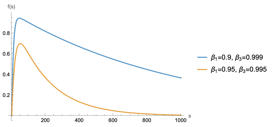 Illustration of gradient weights
In short, the trend is that the farther away, the smaller the coefficient. So in order for the model not to forget any given batch, the coefficient at the farthest point must not be too small. Suppose a coefficient of at least $c \in (0, 1)$ is required for a batch to be remembered; when $s$ is large enough, $\beta_1^s$ first tends to 0, so we have $\beta_3^s - \beta_1^s\approx \beta_3^s$, and solving $\beta_3^s\geq c$ gives $s \leq \frac{\log c}{\log \beta_3} \approx \frac{-\log c}{\lambda\eta}$. This indicates that the model can remember at most $\mathcal{O}(1/\lambda\eta)$ steps' worth of data — this is its memory horizon.
So could we just naively set $\lambda=0$, making the memory horizon infinite, and thereby avoid worrying about forgetting altogether? In theory, yes — but this is not actually a good choice. Weight Decay also serves the purpose of helping the model forget its initialization. From equation $\eqref{eq:theta-0-bar-u}$, we know that the weight of the initialization $\boldsymbol{\theta}_0$ is $\beta_3^t$; if $\beta_3$ is too large, or the number of training steps $t$ is too small, the proportion contributed by the initialization remains high, and the model may still be in an underfitting regime.
Moreover, Weight Decay also helps keep the model's "internal organs" stable. In AdamW's Weight RMS: An Asymptotic Estimate (Part 1)] we already derived that the asymptotic result for AdamW's Weight RMS is $\sqrt{\eta/2\lambda}$; if $\lambda=0$, then the Weight RMS will grow at a rate of $\eta\sqrt{t}$. This means directly setting $\lambda=0$ could also cause weight explosion and other internal pathologies in the model.
Therefore, $\beta_3$ should be neither too small — lest it forget early data — nor too large — lest it lead to underfitting or weight explosion. A reasonably good setting is to make $1/\lambda\eta$ proportional to the number of training steps; in a multi-epoch training scenario, one should instead make $1/\lambda\eta$ proportional to the number of training steps within a single epoch.
The Dynamic Version
In practice, we more commonly use a dynamically varying LR Schedule — Cosine Decay, Linear Decay, WSD (Warmup-Stable-Decay), and so on — so the static Weight Decay and Learning Rate results above don't fully match practice. We need to generalize them to the dynamic case.
Starting from equation $\eqref{eq:wd-ema}$ and using the approximation $1 - \lambda_t \eta_t\approx e^{-\lambda_t \eta_t}$, followed by iterative expansion, we obtain
\begin{equation}\boldsymbol{\theta}_t = (1 - \lambda_t \eta_t)\boldsymbol{\theta}_{t-1} - \eta_t \boldsymbol{u}_t \approx e^{-\lambda_t \eta_t}\boldsymbol{\theta}_{t-1} - \eta_t \boldsymbol{u}_t = e^{-\kappa_t}\left(\boldsymbol{\theta}_0 - \sum_{i=1}^t e^{\kappa_i}\eta_i\boldsymbol{u}_i\right)\end{equation}
where $\kappa_t = \sum_{i=1}^t \eta_i\lambda_i$. Continuing to set $z_t = \sum_{i=1}^t e^{\kappa_i}\eta_i$, we can obtain the same mean-field approximation
\begin{equation}\bar{\boldsymbol{u}}_t\triangleq\frac{1}{z_t}\sum_{i=1}^t e^{\kappa_i}\eta_i \boldsymbol{u}_i = \frac{1}{z_t}\sum_{i=1}^t e^{\kappa_i}\eta_i \frac{\boldsymbol{m}_i}{\sqrt{\boldsymbol{v}_i}}\approx \frac{\bar{\boldsymbol{m}}_t \,\,\triangleq\,\, \frac{1}{z_t}\sum_{i=1}^t e^{\kappa_i}\eta_i\boldsymbol{m}_i}{\sqrt{\bar{\boldsymbol{v}}_t \,\,\triangleq\,\, \frac{1}{z_t}\sum_{i=1}^t e^{\kappa_i}\eta_i\boldsymbol{v}_i}}\end{equation}
Substituting into the expansion of $\boldsymbol{m}_t,\boldsymbol{v}_t$ gives
\begin{gather} \bar{\boldsymbol{m}}_t = \frac{1}{z_t}\sum_{i=1}^t e^{\kappa_i}\eta_i\boldsymbol{m}_i = \frac{1 - \beta_1}{z_t}\sum_{i=1}^t e^{\kappa_i}\eta_i\sum_{j=1}^i \beta_1^{i-j}\boldsymbol{g}_j = \sum_{j=1}^t\boldsymbol{g}_j\underbrace{\frac{1 - \beta_1}{z_t}\sum_{i=j}^t e^{\kappa_i}\beta_1^{i-j}\eta_i}_{\text{denote}\bar{\beta}_1(j,t)} \\ \bar{\boldsymbol{v}}_t = \frac{1}{z_t}\sum_{i=1}^t e^{\kappa_i}\eta_i\boldsymbol{v}_i = \frac{1 - \beta_2}{z_t}\sum_{i=1}^t e^{\kappa_i}\eta_i\sum_{j=1}^i \beta_2^{i-j}\boldsymbol{g}_j^2 = \sum_{j=1}^t\boldsymbol{g}_j^2\underbrace{\frac{1 - \beta_2}{z_t}\sum_{i=j}^t e^{\kappa_i}\beta_2^{i-j}\eta_i}_{\text{denote}\bar{\beta}_2(j,t)} \\ \end{gather}
We can see that compared to the static Weight Decay and Learning Rate case, the dynamic version doesn't change much in form — it's just that the weighting coefficients on the gradients become the slightly more complex $\bar{\beta}_1(j,t)$ and $\bar{\beta}_2(j,t)$. In particular, when $\beta_1,\beta_2\to 0$, $\bar{\beta}_1(j,t)$ and $\bar{\beta}_2(j,t)$ simplify to
\begin{equation}\bar{\beta}_1(j,t) = \bar{\beta}_2(j,t) = \frac{e^{\kappa_j}\eta_j}{z_t}\label{eq:bb1-bb2-0}\end{equation}
Optimal Schedule
There is much more that could be done from here — the most basic being to compute $\bar{\beta}_1(j,t)$ and $\bar{\beta}_2(j,t)$, and estimate the memory horizon, for specific WD and LR Schedules. However, here we choose to do something more ambitious — directly working backward to derive an optimal WD Schedule and LR Schedule.
Specifically, earlier we assumed the data had already been globally shuffled, so every batch's data is equally important. But the coefficient $\bar{\beta}_1(j,t)\propto\beta_3^{t-j+1} - \beta_1^{t-j+1}$ obtained from the static version is not constant — it varies with distance — which doesn't quite match the idea that "every batch's data is equally important." If conditions permit, we would want it to be identically equal to some constant. From this expectation, we can solve backward for the corresponding $\lambda_j,\eta_j$.
For simplicity, let's start from $\beta_1,\beta_2\to 0$. This expected condition can then be written as $\forall 0\leq i,j \leq t, e^{\kappa_i}\eta_i/z_t = e^{\kappa_j}\eta_j/z_t$, which rearranges to $\eta_i / \eta_j = e^{\kappa_j - \kappa_i}$; substituting into $i=j-1$ gives $\eta_{j-1}/\eta_j = e^{\kappa_j - \kappa_{j-1}} = e^{\lambda_j\eta_j}$, or equivalently
\begin{equation}e^{\lambda_j\eta_j}\eta_j = \eta_{j-1}\end{equation}
This gives a numerical method for solving for $\lambda_j,\eta_j$: at each step, once $\eta_{j-1}$ is obtained, $\lambda_j,\eta_j$ can be found next by solving this nonlinear equation, so starting from $\eta_1$ we can recursively obtain the entire sequence. If a more analytical result is desired, we can approximate the difference with a derivative: taking logarithms on both sides gives $\lambda_j\eta_j + \log \eta_j - \log \eta_{j-1} = 0$; treating $\lambda_j,\eta_j$ as a continuous function $\lambda_s,\eta_s$, and $\log \eta_j - \log \eta_{j-1}$ as an approximation to the derivative of $\log \eta_s$, we get
\begin{equation}\lambda_s \eta_s + \frac{\dot{\eta}_s}{\eta_s} \approx 0 \label{eq:lr-wd-ode}\end{equation}
If $\lambda_s$ is taken to be a constant $\lambda$, then we can solve to obtain
\begin{equation}\eta_s \approx \frac{\eta_{\max}}{\lambda\eta_{\max} s + 1}\label{eq:opt-lrt-wd}\end{equation}
This is the optimal LR Schedule under constant Weight Decay. It doesn't require a preset endpoint $t$ or minimum learning rate $\eta_{\min}$, which means it can be trained indefinitely — somewhat like the Stable phase of WSD — but it automatically balances the coefficient of each step's gradient. It does have one drawback, though: as $s\to\infty$, it tends to 0. From AdamW's Weight RMS: An Asymptotic Estimate (Part 2)] we know that the Weight RMS tends to $\lim\limits_{s\to\infty} \frac{\eta_s}{2\lambda_s}$, so this drawback may carry a risk of weight collapse.
To address this issue, we can instead let $\lambda_s = \alpha\eta_s$, with $\alpha=\lambda_{\max}/\eta_{\max}$ a constant, in which case we can solve to obtain
\begin{equation}\eta_s \approx \frac{\eta_{\max}}{\sqrt{2\lambda_{\max}\eta_{\max} s + 1}},\qquad \lambda_s \approx \frac{\lambda_{\max}}{\sqrt{2\lambda_{\max}\eta_{\max} s + 1}} \label{eq:opt-lrt-wdt}\end{equation}
with the corresponding $e^{\kappa_s} \approx \sqrt{2\lambda_{\max}\eta_{\max} s + 1}, e^{\kappa_s}\eta_s \approx \eta_{\max}, z_t\approx \eta_{\max} t, \bar{\beta}_1(j,t) = \bar{\beta}_2(j,t) \approx 1/t$.
General Results
The current results, such as equations $\eqref{eq:opt-lrt-wd}$ and $\eqref{eq:opt-lrt-wdt}$, are all based on $\beta_1,\beta_2=0$. Do the results need to change when these are not zero? More generally, all the results above are based on the Adam optimizer — to what extent can they be generalized to other optimizers?
Let's first look at the case where $\beta_1,\beta_2\neq 0$ is nonzero. The answer is that as long as $t$ is large enough, the conclusions don't need major revision. Taking $\bar{\beta}_1(j,t)$ as an example, under the optimal schedule above $e^{\kappa_i}\eta_i$ equals a constant (related to $t$), so by definition
\begin{equation}\bar{\beta}_1(j,t) = \frac{1 - \beta_1}{z_t}\sum_{i=j}^t e^{\kappa_i}\beta_1^{i-j}\eta_i \propto \sum_{i=j}^t \beta_1^{i-j} = \frac{1 - \beta_1^{t-j+1}}{1 - \beta_1}\end{equation}
When $t$ is large enough, $\beta_1^{t-j+1}\to 0$, so this too can be regarded as a constant independent of $j$. As mentioned earlier, for $\beta_1,\beta_2$, "$t$ being large enough" is almost always guaranteed, so we can just directly use the results for $\beta_1,\beta_2=0$.
As for optimizers, we mentioned earlier SGDM, RMSProp, Adam, SignSGDM, and Muon, which can be divided into two categories. SGDM forms one category on its own — its $\bar{\boldsymbol{u}}_t$ is directly $\bar{\boldsymbol{m}}_t$, without even needing the mean-field approximation, so all the results up through equation $\eqref{eq:lr-wd-ode}$ apply to it. However, equations $\eqref{eq:opt-lrt-wd}$ and $\eqref{eq:opt-lrt-wdt}$ are probably not the most suitable choice for it, because SGDM's asymptotic Weight RMS also depends on the gradient norm see reference ], so the gradient norm needs to be taken into account, making things somewhat more complicated.
The remaining optimizers — RMSProp, Adam, SignSGDM, and Muon — we group into another category, all of which are adaptive-learning-rate optimizers whose update rules all take the homogeneous form $\frac{\text{gradient}}{\sqrt{\text{gradient}{}^2}}$. In this case, if we continue to trust the mean-field approximation, we obtain the same $\bar{\boldsymbol{m}}_t$ and the same $\beta_1(j,t)$, so the results up through equation $\eqref{eq:lr-wd-ode}$ apply here too; and for this class of homogeneous optimizers, one can show that the Weight RMS is likewise asymptotically proportional to $\sqrt{\eta/\lambda}$, so equations $\eqref{eq:opt-lrt-wd}$ and $\eqref{eq:opt-lrt-wdt}$ can also be reused.
Discussion of Assumptions
Our derivation pauses here for now; in this section let's discuss the assumptions the derivation relies on.
Looking back over the whole post, there are two major assumptions worth discussing. The first is the mean-field approximation, first introduced in Rethinking Learning Rate and Batch Size (II): Mean Field]. The mean-field approximation itself is certainly not new — it's a classic approximation from physics — but using it to analyze the dynamics of optimizers appears to be something I introduced myself. So far it has been used to estimate optimizers' Batch Size], Update RMS], and Weight RMS], and the results all seem reasonable.
As for how valid the mean-field approximation really is, there isn't much more I can say — it largely reflects an act of faith. On the one hand, given how reasonable the existing estimation results look, we trust that it will continue to be reasonable, at least giving useful asymptotic estimates for certain scalar quantities. On the other hand, for adaptive-learning-rate optimizers, the nonlinearity of their update rules makes analysis substantially harder, and apart from the mean-field approximation, we really don't have many other computational tools at our disposal.
The most striking example of this is Muon, since its operations are not element-wise, so the component-wise computational tricks that used to work for something like SignSGD lose their effectiveness — yet the mean-field approximation still works (see Rethinking Learning Rate and Batch Size (III): Muon]). So the mean-field approximation effectively provides a unified, effective, and concise computational tool for analyzing and estimating a broad class of adaptive-learning-rate optimizers. There doesn't currently seem to be any other method with the same power, so for now we simply have to keep trusting it.
The second major assumption is that "each step's gradient carries only the information of the current batch." This assumption is, strictly speaking, incorrect, since the gradient depends not only on the current batch's data but also on the previous step's parameters, and those parameters naturally carry historical information. That said, we can try to salvage things somewhat: in theory, every batch should bring some new information — otherwise there would be no reason for that batch to exist — so a fix is to instead assume "each step's gradient carries roughly the same amount of incremental information."
Of course, on closer inspection, even this claim is debatable, since the more the model has already learned and the broader its coverage, the less unique information later batches contribute. Still, we can push a bit further by dividing knowledge into two categories: "patterns/rules" and "facts." Fact-type knowledge — such as who discovered a particular theorem — can only be retained through memorization, so we might refine the assumption to "each step's gradient carries roughly the same amount of fact-type knowledge." In any case, empirically, "treating every step's gradient equally" does seem to yield genuinely beneficial LR Schedules, so it's always worth trying to construct some explanation for it.
A recent paper, How Learning Rate Decay Wastes Your Best Data in Curriculum-Based LLM Pretraining], provides indirect evidence for this. It considers curriculum learning where data quality increases from low to high, and finds that aggressive LR Decay wipes out the advantage of curriculum learning entirely. In our result, the weight of each batch is equation $\eqref{eq:bb1-bb2-0}$, which is proportional to the Learning Rate; if LR Decay is too aggressive, the weight assigned to the higher-quality data that comes later ends up being too small, leading to poor performance. Being able to give a reasonable explanation for this phenomenon in turn supports the plausibility of our assumptions.
Summary
This post approaches Weight Decay (WD) and Learning Rate (LR) from the perspective of exponential moving averages, and explores what the optimal WD Schedule and LR Schedule look like under this perspective.
Translated automatically with claude-sonnet-5; all equations are reproduced verbatim from the source. Copyright remains with the original author.