Why Is Adam's Update RMS 0.2?

为什么Adam的Update RMS是0.2？ 苏剑林 · 2025-09-02 · Mathematics analysis gradient optimizer mean field

As many readers know, we started experimenting with using Muon for large-scale LLM training quite early on. In particular, in Muon Sequel: Why Did We Choose to Try Muon?], we proposed the "Match Adam Update RMS" trick to enable a quick migration from Adam to Muon — a trick that was also used in the training of Kimi K2. This trick consists of unifying Muon's Update RMS to 0.2, which lets us reuse Adam's learning rate and weight decay rate directly.

Behind this trick lies an observation: Adam's Update RMS is approximately 0.2, and this phenomenon is stable and reproducible. This raises an interesting question: why is Adam's Update RMS 0.2? Can we explain it theoretically?

Setting Up the Problem

Let's first describe the phenomenon: from experiments we observe that, roughly speaking, once warmup ends and the model enters the main training phase, Adam's Update RMS stays almost consistently between 0.2 and 0.3, and this pattern holds across models of different sizes. What these models have in common is that they were all trained with Adam, with parameters $\beta_1=0.9,\beta_2=0.95$. Given how consistent this pattern is, it's unlikely to be a coincidence, so I decided to try to analyze the underlying mechanism. more

Let's start by recalling the form of the Adam optimizer:

\begin{equation}\text{Adam}\color{skyblue}{\text{W}}:=\left\{\begin{aligned} &\boldsymbol{m}_t = \beta_1 \boldsymbol{m}_{t-1} + \left(1 - \beta_1\right) \boldsymbol{g}_t\\ &\boldsymbol{v}_t = \beta_2 \boldsymbol{v}_{t-1} + \left(1 - \beta_2\right) \boldsymbol{g}_t^2\\ &\hat{\boldsymbol{m}}_t = \boldsymbol{m}_t\left/\left(1 - \beta_1^t\right)\right.\\ &\hat{\boldsymbol{v}}_t = \boldsymbol{v}_t\left/\left(1 - \beta_2^t\right)\right.\\ &\boldsymbol{u}_t =\hat{\boldsymbol{m}}_t\left/\left(\sqrt{\hat{\boldsymbol{v}}_t} + \epsilon\right)\right.\\ &\boldsymbol{\theta}_t = \boldsymbol{\theta}_{t-1} - \eta_t (\boldsymbol{u}_t \color{skyblue}{ + \lambda_t \boldsymbol{\theta}_{t-1}}) \end{aligned}\right.\end{equation}

Note: throughout this article, all vector multiplications and divisions — including squaring — refer to Hadamard products/quotients, i.e., element-wise operations, unless stated otherwise.

What we want to do is show that $\Vert\boldsymbol{u}_t\Vert_{RMS}\approx 0.2$, at least under the setting $\beta_1=0.9,\beta_2=0.95$. We assume $\epsilon$ is small enough to be negligible, and we consider the steady state of $t\to \infty$, where both $\beta_1^t$ and $\beta_2^t$ are close enough to zero that we needn't distinguish between $\boldsymbol{m}_t$ and $\hat{\boldsymbol{m}}_t$, or between $\boldsymbol{v}_t$ and $\hat{\boldsymbol{v}}_t$. This gives us $\boldsymbol{u}_t =\boldsymbol{m}_t/\sqrt{\boldsymbol{v}_t}$.

For $\boldsymbol{m}_t,\boldsymbol{v}_t$, we can obtain the expansion

\begin{equation}\boldsymbol{m}_t = (1 - \beta_1)\sum_{i=1}^t \beta_1^{t-i}\boldsymbol{g}_i,\qquad \boldsymbol{v}_t = (1 - \beta_2)\sum_{i=1}^t \beta_2^{t-i}\boldsymbol{g}_i^2\end{equation}

Numerical Simulation

If we assume that $\boldsymbol{g}_1,\boldsymbol{g}_2,\cdots,\boldsymbol{g}_t$ are all sampled from the same distribution, then we can estimate $\Vert\boldsymbol{u}_t\Vert_{RMS}$ directly via numerical simulation. Without further ado, let's start with the simplest case — the standard normal distribution $\mathcal{N}(\boldsymbol{0},\boldsymbol{I})$ — using the following reference code:

import numpy as np

N, T = 10000, 2000
beta1, beta2 = 0.9, 0.95
m, v = 0, 0
for t in range(1, T + 1):
    g = np.random.randn(N)
    m = beta1 * m + (1 - beta1) * g
    v = beta2 * v + (1 - beta2) * g**2
    u = m / v**0.5

rms = (u**2).mean()**0.5
print(rms)

Can you guess the result? It comes out to about 0.225, which is remarkably close to the experimental result! This in turn suggests that our simulation assumptions align well with what actually happens in practice. Some readers might object: isn't $\boldsymbol{g}\sim\mathcal{N}(\boldsymbol{0},\boldsymbol{I})$ just pure noise here — how could that possibly match reality? Of course actual training gradients aren't pure noise, but the point is that the signal-to-noise ratio of a single gradient is pitifully small, so modeling it as pure noise is a reasonable approximation.

Readers are welcome to play around with the code above and observe how various factors affect the Update RMS. The general conclusion is: Update RMS is positively correlated with $\beta_1$, seems largely unrelated to $\beta_2$, and if the distribution of $\boldsymbol{g}$ has a nonzero mean (equivalent to increasing the gradient's signal-to-noise ratio), then the Update RMS also increases.

Mean-Field Approximation

In this section I'll attempt to derive an approximate analytical solution for the simulation result above from a theoretical angle. First, from the definition of RMS, to compute $\Vert\boldsymbol{u}_t\Vert_{RMS}$ we first need $\boldsymbol{u}_t^2 = \boldsymbol{m}_t^2/\boldsymbol{v}_t$. My idea is to use the expectation of $\boldsymbol{u}_t^2$ as an approximation for it, and further convert this into a mean-field approximation:

\begin{equation}\mathbb{E}[\boldsymbol{u}_t^2] = \mathbb{E}\left[\frac{\boldsymbol{m}_t^2}{\boldsymbol{v}_t}\right] \approx \frac{\mathbb{E}[\boldsymbol{m}_t^2]}{\mathbb{E}[\boldsymbol{v}_t]}\end{equation}

Some readers may question the validity of the last approximation step. My suggestion is: let's set aside these details for now, just as we assumed $\boldsymbol{g}\sim\mathcal{N}(\boldsymbol{0},\boldsymbol{I})$ in the previous section — compute first, question later. If the result turns out reasonable, then the process is presumably reasonable to some extent as well. Let's now compute the numerator and denominator separately; this time we set $\mathbb{E}[\boldsymbol{g}]=\boldsymbol{\mu},\mathbb{E}[\boldsymbol{g}^2]=\boldsymbol{\mu}^2 + \boldsymbol{\sigma}^2 $ in general, where the denominator is relatively simple:

\begin{equation}\begin{aligned} \mathbb{E}[\boldsymbol{v}_t] =&\, (1 - \beta_2)\sum_{i=1}^t \beta_2^{t-i}\mathbb{E}[\boldsymbol{g}_i^2] \\ =&\, (1 - \beta_2)\sum_{i=1}^t \beta_2^{t-i}(\boldsymbol{\mu}^2 + \boldsymbol{\sigma}^2) \\ =&\, (1 - \beta_2^t) (\boldsymbol{\mu}^2 + \boldsymbol{\sigma}^2) \\[5pt] \approx &\, \boldsymbol{\mu}^2 + \boldsymbol{\sigma}^2 \qquad(t\to\infty) \end{aligned}\end{equation}

As for the numerator, we can either expand the square directly, or take a slight shortcut: what we want is the second moment $\boldsymbol{m}_t$, namely $\mathbb{E}[\boldsymbol{m}_t^2]$, which in turn equals $\mathbb{E}[\boldsymbol{m}_t]^2 + \mathbb{V}ar[\boldsymbol{m}_t]$. The computation of $\mathbb{E}[\boldsymbol{m}_t]$ is similar to that of $\mathbb{E}[\boldsymbol{m}_t]$, giving the result $(1 - \beta_1^t)\boldsymbol{\mu}\approx\boldsymbol{\mu}$; as for the variance, it is additive under summation, so

\begin{equation}\mathbb{V}ar[\boldsymbol{m}_t] = (1 - \beta_1)^2\sum_{i=1}^t \beta_1^{2(t-i)}\boldsymbol{\sigma}^2 = \frac{(1 - \beta_1)^2 (1 - \beta_1^{2t})}{1 - \beta_1^2}\boldsymbol{\sigma}^2\approx \frac{1 - \beta_1}{1 + \beta_1}\boldsymbol{\sigma}^2\qquad (t\to\infty)\end{equation}

Therefore

\begin{equation}\mathbb{E}[\boldsymbol{u}_t^2]\approx \frac{\boldsymbol{\mu}^2 + \frac{1 - \beta_1}{1 + \beta_1}\boldsymbol{\sigma}^2}{\boldsymbol{\mu}^2 + \boldsymbol{\sigma}^2}\end{equation}

Analyzing the Result

Since $\mathbb{E}[\boldsymbol{u}_t^2]$ is already a squared vector, to estimate $\Vert\boldsymbol{u}_t\Vert_{RMS}$ we simply need to average over its components and then take the square root. For this averaging step, let's apply the mean-field approximation once more (averaging numerator and denominator separately), and we finally arrive at

\begin{equation}\Vert\boldsymbol{u}_t\Vert_{RMS} \approx \sqrt{\frac{\Vert\boldsymbol{\mu}\Vert^2 + \frac{1 - \beta_1}{1 + \beta_1}\Vert\boldsymbol{\sigma}\Vert^2}{\Vert\boldsymbol{\mu}\Vert^2 + \Vert\boldsymbol{\sigma}\Vert^2}} = \sqrt{\frac{\Vert\boldsymbol{\mu}\Vert^2/\Vert\boldsymbol{\sigma}\Vert^2 + \frac{1 - \beta_1}{1 + \beta_1}}{\Vert\boldsymbol{\mu}\Vert^2/\Vert\boldsymbol{\sigma}\Vert^2 + 1}}\label{eq:mean-field}\end{equation}

There are two factors influencing this result: one is $\Vert\boldsymbol{\mu}\Vert^2/\Vert\boldsymbol{\sigma}\Vert^2$, which can be viewed as the signal-to-noise ratio (SNR) of the gradient; the other is $\beta_1$, one of Adam's hyperparameters. Notably, the result doesn't depend on $\beta_2$, which matches our earlier simulation results. So how good is this approximation, actually? Let's consider the simplest special case, $\boldsymbol{\mu}=\boldsymbol{0}$, in which case

\begin{equation}\Vert\boldsymbol{u}_t\Vert_{RMS} \approx \sqrt{\frac{1 - \beta_1}{1 + \beta_1}}\end{equation}

Substituting $\beta_1=0.9$ gives the result $0.2294\cdots$, which — remarkably — matches both the simulation results and empirical behavior quite well! Furthermore, here's a more detailed comparison against the simulation results:

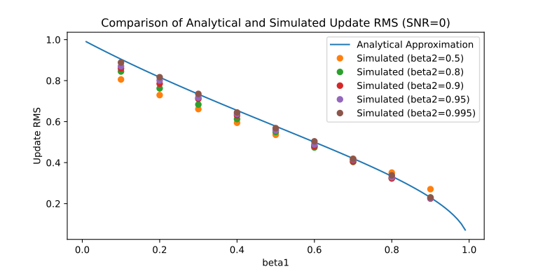] Comparison of simulation results and mean-field approximation (varying beta1, beta2)

Overall, the approximation holds up quite well, especially once $\beta_2 \geq 0.9$ — after which the results almost coincide with the mean-field approximation (thanks to @EIFY] for pointing out that the paper Rotational Equilibrium: How Weight Decay Balances Learning Across Neural Networks] arrived at the same computational result previously).

As for the comparison taking SNR into account, the results are as follows:

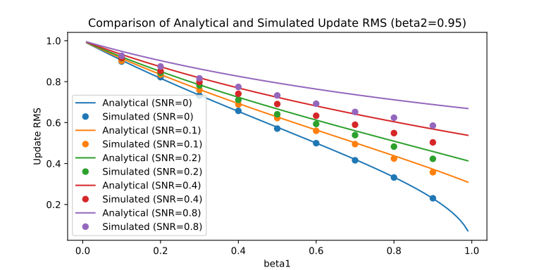] Comparison of simulation results and mean-field approximation (varying beta1, SNR)

As the signal-to-noise ratio increases, the error of the mean-field approximation grows, though it can still predict the overall trend. In fact, in real training the gradient's signal-to-noise ratio rarely gets anywhere close to 1, so the mean-field approximation can still be considered a good fit.

Working Backward

If we accept the mean-field approximation $\eqref{eq:mean-field}$, then we can use it in reverse to estimate the gradient's signal-to-noise ratio:

\begin{equation}\frac{\Vert\boldsymbol{\mu}\Vert^2}{\Vert\boldsymbol{\sigma}\Vert^2} \approx \frac{\Vert\boldsymbol{u}_t\Vert_{RMS}^2 - \frac{1 - \beta_1}{1 + \beta_1}}{1 - \Vert\boldsymbol{u}_t\Vert_{RMS}^2}\end{equation}

In actual training, $\beta_1$ is given, and $\Vert\boldsymbol{u}_t\Vert_{RMS}$ (i.e., Adam's Update RMS) can also be estimated directly, so the above expression is computable. Of course, this formula only applies to Adam — is there a more general estimation approach? As it turns out, there is! Recall that we earlier estimated

\begin{equation}\mathbb{E}[\boldsymbol{m}_t^2]\approx \boldsymbol{\mu}^2 + \frac{1 - \beta_1}{1 + \beta_1}\boldsymbol{\sigma}^2\end{equation}

If we sum over its components and take the square root, we can regard the result as an approximation of $\Vert\boldsymbol{m}_t\Vert$:

\begin{equation}\Vert\boldsymbol{m}_t\Vert\approx \sqrt{\Vert\boldsymbol{\mu}\Vert^2 + \frac{1 - \beta_1}{1 + \beta_1}\Vert\boldsymbol{\sigma}\Vert^2}\end{equation}

As for the second moment, it is $\mathbb{E}[\boldsymbol{v}_t]\approx \boldsymbol{\mu}^2 + \boldsymbol{\sigma}^2$; but optimizers like Muon don't have a second moment to work with. However, we notice that the result for the second moment doesn't depend on $\beta_2$, so let's consider the simplest special case — $\beta_2=0$ — in which case $\boldsymbol{v}_t=\boldsymbol{g}_t^2$. This might feel like a bit of a stretch, but when it comes to estimation, we go with whatever is convenient. This "approximation" amounts to assuming $\Vert\boldsymbol{g}_t\Vert^2\approx \Vert\boldsymbol{\mu}\Vert^2 + \Vert\boldsymbol{\sigma}\Vert^2$ holds, so we get

\begin{equation}\frac{\Vert\boldsymbol{m}_t\Vert}{\Vert\boldsymbol{g}_t\Vert}\approx \sqrt{\frac{\Vert\boldsymbol{\mu}\Vert^2 + \frac{1 - \beta_1}{1 + \beta_1}\Vert\boldsymbol{\sigma}\Vert^2}{\Vert\boldsymbol{\mu}\Vert^2 + \Vert\boldsymbol{\sigma}\Vert^2}}\end{equation}

The form of the right-hand side is exactly the same as in equation $\eqref{eq:mean-field}$, so we can write

\begin{equation}\frac{\Vert\boldsymbol{\mu}\Vert^2}{\Vert\boldsymbol{\sigma}\Vert^2} \approx \frac{\Vert\boldsymbol{m}_t\Vert^2/\Vert\boldsymbol{g}_t\Vert^2 - \frac{1 - \beta_1}{1 + \beta_1}}{1 - \Vert\boldsymbol{m}_t\Vert^2/\Vert\boldsymbol{g}_t\Vert^2}\end{equation}

That is, by substituting $\Vert\boldsymbol{m}_t\Vert/\Vert\boldsymbol{g}_t\Vert$ for $\Vert\boldsymbol{u}_t\Vert_{RMS}$, we obtain a general approach for estimating $\Vert\boldsymbol{\mu}\Vert^2/\Vert\boldsymbol{\sigma}\Vert^2$ that applies to any optimizer with momentum. Some readers might ask: what if there's no momentum at all? In that case, there's really nothing we can do, because $\Vert\boldsymbol{\mu}\Vert^2/\Vert\boldsymbol{\sigma}\Vert^2$ here is a statistic that spans the entire optimization trajectory — we need some cross-trajectory statistical information in order to estimate it.

Summary

This article explored Adam's Update RMS from two angles — numerical simulation and theoretical approximation — providing one theoretical justification for our choice to align Muon's Update RMS to 0.2.