How does Adam's epsilon affect the learning rate Scaling Law?
In the previous post 《When Batch Size Grows, How Should the Learning Rate Change Accordingly?》] we discussed the scaling relationship between learning rate and batch size from several angles; for the Adam optimizer we used the SignSGD approximation, which is a common device for analyzing Adam. A natural question then arises: just how scientifically sound is it to approximate Adam by SignSGD?
As we know, the denominator of Adam's update contains an $\epsilon$, originally introduced to prevent division by zero, so its value is usually taken to be very close to zero, to the point that we typically choose to ignore it in theoretical analysis. However, in current LLM training—especially low-precision training—we tend to choose a relatively large $\epsilon$, which means that during the middle and late stages of training $\epsilon$ often already exceeds the magnitude of the squared gradient, so the presence of $\epsilon$ can no longer be neglected in practice.
Therefore, in this post we try to explore how $\epsilon$ affects the Scaling Law between Adam's learning rate and batch size, offering a reference computation scheme for this problem.more
SoftSign
Since this continues directly from the previous post, I won't repeat the background here. To investigate the role of $\epsilon$, we switch from SignSGD to SoftSignSGD, i.e., $\newcommand{sign}{\mathop{\text{sign}}}\tilde{\boldsymbol{\varphi}}_B = \sign(\tilde{\boldsymbol{g}}_B)$ becomes $\tilde{\boldsymbol{\varphi}}_B = \text{softsign}(\tilde{\boldsymbol{g}}_B)$, where
\begin{equation}\sign(x)=\frac{x}{\sqrt{x^2}}\quad\to\quad\text{softsign}(x, \epsilon)=\frac{x}{\sqrt{x^2+\epsilon^2}}\end{equation}
This form is undoubtedly closer to Adam. But before proceeding, we need to confirm whether $\epsilon$ is really non-negligible, in order to decide whether further investigation is worthwhile.
In Keras's implementation of Adam, the default value of $\epsilon$ is $10^{-7}$, while in Torch it is $10^{-8}$; in this case the probability that the absolute value of the gradient is smaller than $\epsilon$ isn't particularly large. But in LLMs, the commonly used value of $\epsilon$ is $10^{-5}$ (as in LLAMA2]), and once training enters its "steady phase," components with gradient absolute value smaller than $\epsilon$ become quite common, so the effect of $\epsilon$ is significant.
This is also related to the parameter count of the LLM. For a model that trains stably, regardless of its parameter count, the magnitude of its gradient norm generally stays on the same order of magnitude—this is dictated by the stability requirements of backpropagation (see 《What exactly makes training a 1000-layer Transformer difficult?》]). Consequently, the larger the model's parameter count, the smaller the average absolute gradient value per parameter becomes, which makes the role of $\epsilon$ even more pronounced.
It's worth pointing out that introducing $\epsilon$ effectively provides an interpolation between Adam and SGD, because when $x\neq 0$,
\begin{equation}\lim_{\epsilon\to \infty}\epsilon\,\text{softsign}(x, \epsilon)=\lim_{\epsilon\to \infty}\frac{x \epsilon}{\sqrt{x^2+\epsilon^2}} = x\end{equation}
So the larger $\epsilon$ is, the more Adam's behavior resembles SGD.
S-shaped approximations
Having confirmed the necessity of introducing $\epsilon$, let's proceed with the analysis. Along the way we will repeatedly encounter S-shaped (sigmoid-like) functions, so as a preparatory step we should also look into simple approximations of such functions.
S-shaped functions are nothing new to readers by now—the $\text{softsign}$ function introduced in the previous section is itself one example, as is the $\text{erf}$ function used in the analysis in the previous post, along with others such as $\tanh$ and $\text{sigmoid}$. What we'll deal with next is an S-shaped function $S(x)$ satisfying the following properties:
1. globally smooth and monotonically increasing;
2. an odd function with range $[-1,1]$;
3. slope $k > 0$ at the origin.
For this class of functions, we consider two approximations. The first is analogous to $\text{softsign}$:
\begin{equation}S(x)\approx \frac{x}{\sqrt{x^2 + 1/k^2}}\end{equation}
This is arguably the simplest function that retains the above three properties of $S(x)$. The second approximation is based on the $\text{clip}$ function:
\begin{equation}S(x)\approx \text{clip}(kx, -1, 1) \triangleq \left\{\begin{aligned}&1, &kx\geq 1 \\ &kx, &-1 < kx < 1\\ &-1, &kx \leq -1\end{aligned}\right.\end{equation}
This is essentially a piecewise-linear function, which gives up global smoothness, but the piecewise-linear structure makes the resulting integrals much easier to compute, as we'll soon see.
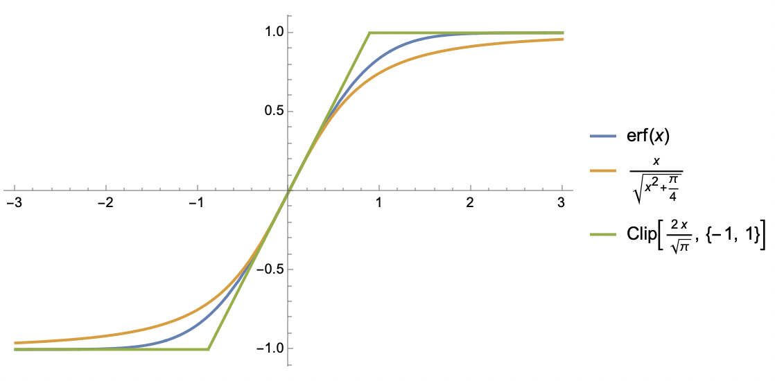 The Erf function and its two approximations
Estimating the mean
Without further ado, following the approach of the previous post, our starting point is still
\begin{equation}\mathbb{E}[\mathcal{L}(\boldsymbol{w} - \eta\tilde{\boldsymbol{\varphi}}_B)] \approx \mathcal{L}(\boldsymbol{w}) - \eta\mathbb{E}[\tilde{\boldsymbol{\varphi}}_B]^{\top}\boldsymbol{g} + \frac{1}{2}\eta^2 \text{Tr}(\mathbb{E}[\tilde{\boldsymbol{\varphi}}_B\tilde{\boldsymbol{\varphi}}_B^{\top}]\boldsymbol{H})\end{equation}
What we need to do is estimate $\mathbb{E}[\tilde{\boldsymbol{\varphi}}_B]$ and $\mathbb{E}[\tilde{\boldsymbol{\varphi}}_B\tilde{\boldsymbol{\varphi}}_B^{\top}]$.
In this section we compute $\mathbb{E}[\tilde{\boldsymbol{\varphi}}_B]$, for which we need to approximate the $\text{softsign}$ function using the $\text{clip}$ function:
\begin{equation}\text{softsign}(x, \epsilon)\approx \text{clip}(x/\epsilon, -1, 1) = \left\{\begin{aligned}&1, & x/\epsilon \geq 1 \\ & x / \epsilon, & -1 < x/\epsilon < 1 \\ &-1, & x/\epsilon \leq -1 \\ \end{aligned}\right.\end{equation}
We then have
\begin{equation}\begin{aligned} \mathbb{E}[\tilde{\varphi}_B] =&\, \mathbb{E}[\text{softsign}(g + \sigma z/\sqrt{B}, \epsilon)] \approx \mathbb{E}[\text{clip}(g/\epsilon + \sigma z/\epsilon\sqrt{B},-1, 1)] \\[5pt] =&\,\frac{1}{\sqrt{2\pi}}\int_{-\infty}^{\infty} \text{clip}(g/\epsilon + \sigma z/\epsilon\sqrt{B},-1, 1) e^{-z^2/2}dz \\[5pt] =&\,\frac{1}{\sqrt{2\pi}}\int_{-\infty}^{-(g+\epsilon)\sqrt{B}/\sigma} (-1)\times e^{-z^2/2}dz + \frac{1}{\sqrt{2\pi}}\int_{-(g-\epsilon)\sqrt{B}/\sigma}^{\infty} 1\times e^{-z^2/2}dz \\[5pt] &\,\qquad\qquad + \frac{1}{\sqrt{2\pi}}\int_{-(g+\epsilon)\sqrt{B}/\sigma}^{-(g-\epsilon)\sqrt{B}/\sigma} (g/\epsilon + \sigma z/\epsilon\sqrt{B})\times e^{-z^2/2}dz \end{aligned}\end{equation}
The integral expression is quite complicated, but it's not hard to compute with Mathematica, and the result can be expressed using the $\text{erf}$ function:
\begin{equation}\frac{1}{2}\left[\text{erf}\left(\frac{a+b}{\sqrt{2}}\right)+\text{erf}\left(\frac{a-b}{\sqrt{2}}\right)\right]+\frac{a}{2b}\left[\text{erf}\left(\frac{a+b}{\sqrt{2}}\right)-\text{erf}\left(\frac{a-b}{\sqrt{2}}\right)\right]+\frac{e^{-(a+b)^2/2} - e^{-(a-b)^2/2}}{b\sqrt{2\pi}}\end{equation}
where $a = g\sqrt{B}/\sigma, b=\epsilon \sqrt{B}/\sigma$. This function looks fairly complicated, but it happens to be an S-shaped function of $a$, with range $(-1,1)$ and slope $\text{erf}(b/\sqrt{2})/b$ at $a=0$, so we can use the first form of approximation
\begin{equation}\mathbb{E}[\tilde{\varphi}_B]\approx\frac{a}{\sqrt{a^2 + b^2 / \text{erf}(b/\sqrt{2})^2}}\approx \frac{a}{\sqrt{a^2 + b^2 + \pi / 2}}=\frac{g/\sigma}{\sqrt{(g^2+\epsilon^2)/\sigma^2 + \pi / 2B}}\label{eq:E-u-approx}\end{equation}
The second approximate-equality sign uses the approximation $\text{erf}(x)\approx x / \sqrt{x^2 + \pi / 4}$ to handle the $\text{erf}(b/\sqrt{2})$ in the denominator. Quite fortunately, the final form isn't overly complicated. Next we have
\begin{equation}\mathbb{E}[\tilde{\boldsymbol{\varphi}}_B]_i \approx \frac{g_i/\sigma_i}{\sqrt{(g_i^2+\epsilon^2)/\sigma_i^2 + \pi / 2B}} = \frac{\text{softsign}(g_i, \epsilon)}{\sqrt{1 + \pi \sigma_i^2 /(g_i^2+\epsilon^2)/2B}}\approx \frac{\text{softsign}(g_i, \epsilon)}{\sqrt{1 + \pi \kappa^2/2B}} = \nu_i \beta\end{equation}
As in the previous post, the last approximate-equality sign uses the mean-field approximation, where $\kappa^2$ is some average of all the $\sigma_i^2 /(g_i^2+\epsilon^2)$, and $\nu_i = \text{softsign}(g_i, \epsilon)$ and $\beta = (1 + \pi\kappa^2 / 2B)^{-1/2}$.
Estimating the variance
With the mean, i.e. the first moment, taken care of, now it's the turn of the second moment
\begin{equation}\begin{aligned} \mathbb{E}[\tilde{\varphi}_B^2] =&\, \mathbb{E}[\text{softsign}(g + \sigma z/\sqrt{B}, \epsilon)^2] \approx \mathbb{E}[\text{clip}(g/\epsilon + \sigma z/\epsilon\sqrt{B},-1, 1)^2] \\[5pt] =&\,\frac{1}{\sqrt{2\pi}}\int_{-\infty}^{\infty} \text{clip}(g/\epsilon + \sigma z/\epsilon\sqrt{B},-1, 1)^2 e^{-z^2/2}dz \\[5pt] =&\,\frac{1}{\sqrt{2\pi}}\int_{-\infty}^{-(g+\epsilon)\sqrt{B}/\sigma} (-1)^2\times e^{-z^2/2}dz + \frac{1}{\sqrt{2\pi}}\int_{-(g-\epsilon)\sqrt{B}/\sigma}^{\infty} 1^2\times e^{-z^2/2}dz \\[5pt] &\,\qquad\qquad + \frac{1}{\sqrt{2\pi}}\int_{-(g+\epsilon)\sqrt{B}/\sigma}^{-(g-\epsilon)\sqrt{B}/\sigma} (g/\epsilon + \sigma z/\epsilon\sqrt{B})^2\times e^{-z^2/2}dz \end{aligned}\end{equation}
The result can likewise be expressed using the $\text{erf}$ function, but it's much more verbose, so we won't write it out here—again, this is no trouble for Mathematica. Viewed as a function of $a$, one finds that the result traces an inverted bell-shaped curve, symmetric about the $y$ axis, with upper bound $1$, and a minimum located within $(0,1)$. Referring to the approximation $\eqref{eq:E-u-approx}$ for $\mathbb{E}[\tilde{\varphi}_B]$, we choose the following approximation
\begin{equation}\mathbb{E}[\tilde{\varphi}_B^2] \approx 1 - \frac{b^2}{a^2 + b^2 + \pi / 2} = 1 - \frac{\epsilon^2/(g^2+\epsilon^2)}{1 + \pi\sigma^2/(g^2+\epsilon^2) / 2B}\end{equation}
To be honest, this approximation isn't very precise—it's chosen mainly for computational convenience—but it retains the key features: the inverted bell shape, symmetry about the $y$ axis, upper bound of 1, a value of 1 at $b=0$, and a value of 0 at $b\to\infty$. Continuing to apply the mean-field approximation:
\begin{equation}\mathbb{E}[\tilde{\boldsymbol{\varphi}}_B\tilde{\boldsymbol{\varphi}}_B^{\top}]_{i,i} \approx 1 - \frac{\epsilon^2/(g_i^2+\epsilon^2)}{1 + \pi\sigma_i^2/(g_i^2+\epsilon^2) / 2B}\approx 1 - \frac{\epsilon^2/(g_i^2+\epsilon^2)}{1 + \pi\kappa^2 / 2B} = \nu_i^2 \beta^2 + (1 - \beta^2)\end{equation}
Hence $\mathbb{E}[\tilde{\boldsymbol{\varphi}}_B\tilde{\boldsymbol{\varphi}}_B^{\top}]_{i,j}\approx \nu_i \nu_j \beta^2 + \delta_{i,j}(1-\beta^2)$. Here the term $\delta_{i,j}(1-\beta^2)$ represents the covariance matrix $(1-\beta^2)\boldsymbol{I}$ of $\tilde{\boldsymbol{\varphi}}$, which is a diagonal matrix—unsurprisingly, since one of our assumptions is that the components of $\tilde{\boldsymbol{\varphi}}$ are independent of each other, so the covariance matrix must indeed be diagonal.
A first look at the result
From this we obtain
\begin{equation}\eta^* \approx \frac{\mathbb{E}[\tilde{\boldsymbol{\varphi}}_B]^{\top}\boldsymbol{g}}{\text{Tr}(\mathbb{E}[\tilde{\boldsymbol{\varphi}}_B\tilde{\boldsymbol{\varphi}}_B^{\top}]\boldsymbol{H})} \approx \frac{\beta\sum_i \nu_i g_i}{\beta^2\sum_{i,j} \nu_i \nu_j H_{i,j} + (1-\beta^2)\sum_i H_{i,i} }\end{equation}
Note that apart from $\beta$, none of the remaining symbols depend on $B$, so the expression above already gives us the dependence between $\eta^*$ and $B$. Note also that, to guarantee the existence of a minimum, we always assume positive-definiteness of the $\boldsymbol{H}$ matrix, under which assumption we necessarily have $\sum_{i,j} \nu_i \nu_j H_{i,j} > 0$ and $\sum_i H_{i,i} > 0$.
In the previous post we noted that the most notable feature of Adam is the possible appearance of a "Surge phenomenon," i.e., $\eta^*$ ceasing to be a globally monotonically increasing function of $B$. We will now show that introducing $\epsilon > 0$ reduces the probability of the Surge phenomenon occurring, and it disappears entirely when $\epsilon \to \infty$. The proof is not difficult: it's clear that a necessary condition for the Surge phenomenon to occur is
\begin{equation}\sum_{i,j} \nu_i \nu_j H_{i,j} - \sum_i H_{i,i} > 0\end{equation}
If this fails, then the whole of $\eta^*$ is monotonically increasing in $\beta$, and since $\beta$ is monotonically increasing in $B$, the whole of $\eta^*$ is monotonically increasing in $B$, so there's no Surge phenomenon. Recall that $\nu_i = \text{softsign}(g_i, \epsilon)$ is a monotonically decreasing function of $\epsilon$, so as $\epsilon$ increases, $\sum_{i,j} \nu_i \nu_j H_{i,j}$ becomes smaller, making it less likely for the above inequality to hold; and when $\epsilon\to \infty$, $\nu_i$ becomes zero, so the inequality can no longer hold at all, and the Surge phenomenon disappears entirely.
Furthermore, we can show that when $\epsilon\to\infty$, the result coincides with that of SGD, which just requires noting that
\begin{equation}\frac{\eta^*}{\epsilon} \approx \frac{\beta\sum_i (\epsilon \nu_i) g_i}{\beta^2\sum_{i,j} (\epsilon \nu_i)(\epsilon \nu_j) H_{i,j} + \epsilon^2(1-\beta^2)\sum_i H_{i,i} }\end{equation}
we have the limit
\begin{equation}\lim_{\epsilon\to\infty} \beta = 1,\quad\lim_{\epsilon\to\infty} \epsilon \nu_i = g_i, \quad \lim_{\epsilon\to\infty} \epsilon^2(1-\beta^2) = \pi \sigma^2 / 2B\end{equation}
Here $\sigma^2$ is some average of all the $\sigma_i^2$. Thus, for sufficiently large $\epsilon$, we obtain the approximation
\begin{equation}\frac{\eta^*}{\epsilon} \approx \frac{\sum_i g_i^2}{\sum_{i,j} g_i g_j H_{i,j} + \left(\pi \sigma^2\sum_i H_{i,i}\right)/2B }\end{equation}
where the right-hand side is precisely the SGD result under the assumption that the gradient covariance matrix is $(\pi\sigma^2/2B)\boldsymbol{I}$.
Summary
This post continues the approach of the previous one, attempting to analyze how Adam's $\epsilon$ affects the Scaling Law between learning rate and batch size. The result takes a form interpolating between SGD and SignSGD: the larger $\epsilon$ is, the closer the result gets to SGD, and the lower the probability of the "Surge phenomenon" appearing. On the whole, the computed result contains no especially surprising elements, but it can serve as a useful reference for analyzing the role of $\epsilon$.
Translated automatically with claude-sonnet-5; all equations are reproduced verbatim from the source. Copyright remains with the original author.