Aligning with Full Fine-Tuning! The Most Impressive LoRA Improvement I've Seen (Part 1)
As we all know, LoRA is a common parameter-efficient fine-tuning method, which we gave a brief introduction to in LoRA from a Gradient Perspective: Introduction, Analysis, Speculation, and Generalization. LoRA uses low-rank decomposition to reduce the number of fine-tuning parameters and save fine-tuning GPU memory, while the trained weights can be merged back into the original weights, meaning the inference architecture doesn't need to change — it's a fine-tuning approach that's friendly to both training and inference. In addition, in Setting Different Learning Rates — Can LoRA Improve Even Further? we also discussed the asymmetry in LoRA, pointing out that setting different learning rates for $A,B$ can achieve better results, a conclusion known as "LoRA+".
To further improve performance, researchers have proposed quite a few other LoRA variants, such as AdaLoRA, rsLoRA, DoRA, PiSSA, and so on. These modifications all make some sense, but none of them left a particularly deep impression. However, the recent paper LoRA-GA: Low-Rank Adaptation with Gradient Approximation caught my eye — just skimming the abstract already gave me the feeling that it simply had to work, and after reading it carefully I found it to be the most impressive LoRA improvement to date.
So just how impressive is it exactly? How much is LoRA-GA actually worth? Let's take a look together.more
A Quick Recap
Let's first review LoRA. Suppose the pretrained parameters are $W_0 \in \mathbb{R}^{n\times m}$; then the update during full fine-tuning is naturally also a $n\times m$ matrix. LoRA constrains this update to be a low-rank matrix in order to reduce the number of trainable parameters, i.e., it sets $W=W_0 + AB$, where $A\in\mathbb{R}^{n\times r},B\in\mathbb{R}^{r\times m}$ and $r\ll \min(n,m)$. It then replaces the original model parameters with the new $W$, keeping $W_0$ fixed and training only $A,B$, as shown in the figure below:
$$\style{display: inline-block; width: 24ex; padding: 10ex 0; border: 1px solid #6C8EBF; background-color: #DAE8FC}{W_0\in\mathbb{R}^{n\times m}} \quad + \quad \style{display: inline-block; width: 8ex; padding: 10ex 0; border: 1px solid #D79B00; background-color: #FFE6CC}{A\in\mathbb{R}^{n\times r}}\quad\times\quad \style{display: inline-block; width: 24ex; padding: 3ex 0; border: 1px solid #D79B00; background-color: #FFE6CC}{B\in\mathbb{R}^{r\times m}}$$
To make LoRA's initial state consistent with the pretrained model, we usually initialize one of $A,B$ to all zeros, which gives us $A_0 B_0=0$, so that the initial $W$ is exactly $W_0$. But this isn't strictly necessary — if $A,B$ are both initialized to non-zero values, we can instead set $W$ to
\begin{equation}W = (W_0 - A_0 B_0) + AB\end{equation}
In other words, by changing the fixed weight from $W_0$ to $W_0 - A_0 B_0$, we can still satisfy the condition that the initial $W$ equals $W_0$.
It should be pointed out that LoRA is often just a reluctant compromise made when GPU memory is insufficient, since in general full fine-tuning outperforms LoRA. So if you have enough compute and want the best possible results, full fine-tuning should be your first choice. This is in fact one of the assumptions underlying LoRA-GA, since its direction of improvement is precisely to align with full fine-tuning. Another scenario where LoRA is used is when there are large numbers of small customization needs and we need to store many sets of fine-tuning results — in this case LoRA reduces storage costs.
Aligning with Full Fine-Tuning
LoRA-GA proposes a remarkably deep optimization insight: through $W=(W_0 - A_0 B_0) + AB$ we can guarantee that the initial value of $W$ equals $W_0$, i.e., that in its initial state, LoRA is equivalent to full fine-tuning. Given this, can we also adjust $A_0$ and $B_0$ so that LoRA and full fine-tuning remain as similar as possible during subsequent training? For instance, in the simplest case, can we make $W_1$ after the first optimization step as close as possible?
The more you turn this idea over, the more you realize it "cuts straight to the essence" — isn't the whole point of LoRA to "achieve a lot with a little," hoping to get as close as possible to the effectiveness of full fine-tuning? If so, then aligning the subsequent update results with full fine-tuning as closely as possible is surely the most correct direction for improvement. From an approximation standpoint, "the initial value of $W$ equals $W_0$" corresponds to a zeroth-order approximation of full fine-tuning, while keeping the subsequent $W_1,W_2,\cdots$ close corresponds to a higher-order approximation — a perfectly reasonable choice. So after reading the abstract, I had a strong feeling of "this is it."
Specifically, suppose our optimizer is SGD. Then for full fine-tuning we have
\begin{equation} W_1 = W_0 - \eta \frac{\partial \mathcal{L}}{\partial W_0}\end{equation}
where $\mathcal{L}$ is the loss function and $\eta$ is the learning rate. For LoRA, we have
\begin{equation}\begin{gathered} A_1 = A_0 - \eta \frac{\partial \mathcal{L}}{\partial A_0} = A_0 - \eta \frac{\partial \mathcal{L}}{\partial W_0} B_0^{\top},\quad B_1 = B_0 - \eta \frac{\partial \mathcal{L}}{\partial B_0} = B_0 - \eta A_0^{\top}\frac{\partial \mathcal{L}}{\partial W_0} \\[8pt] W_1 = W_0 - A_0 B_0 + A_1 B_1 \approx W_0 - \eta\left(A_0 A_0^{\top}\frac{\partial \mathcal{L}}{\partial W_0} + \frac{\partial \mathcal{L}}{\partial W_0}B_0^{\top} B_0\right) \end{gathered}\end{equation}
where the final approximation drops the second-order term in $\eta$. Now the two $W_1$ have similar forms, and to make them as close as possible, we can consider minimizing
\begin{equation}\mathop{\text{argmin}}_{A_0,B_0}\left\Vert A_0 A_0^{\top}\frac{\partial \mathcal{L}}{\partial W_0} + \frac{\partial \mathcal{L}}{\partial W_0}B_0^{\top} B_0 - \frac{\partial \mathcal{L}}{\partial W_0}\right\Vert_F^2 \label{eq:loss-0}\end{equation}
where $\Vert\cdot\Vert_F^2$ denotes the square of the matrix's Frobenius norm, i.e., the sum of squares of every element of the matrix.
The Solution Process
For simplicity, let's write $G_0=\frac{\partial \mathcal{L}}{\partial W_0}$, so that the objective $\eqref{eq:loss-0}$ can be abbreviated as
\begin{equation}\mathop{\text{argmin}}_{A_0,B_0}\left\Vert A_0 A_0^{\top}G_0 + G_0 B_0^{\top} B_0 - G_0\right\Vert_F^2 \label{eq:loss-1}\end{equation}
Note that both $A_0 A_0^{\top}G_0$ and $G_0 B_0^{\top} B_0$ have rank at most $r$, so their sum has rank at most $2r$; assuming $2r < \min(n,m)$, the objective above amounts to finding the best rank-$2r$-or-lower approximation of $G_0$.
Let's first consider the case where $G_0$ is a non-negative diagonal matrix, with the diagonal entries already sorted in decreasing order. This case is straightforward: its best approximation of rank at most $2r$ is simply the new diagonal matrix that keeps only the first $2r$ diagonal entries. This result is known as the "Eckart–Young–Mirsky theorem," and one choice of $A_0,B_0$ that makes $A_0 A_0^{\top}G_0 + G_0 B_0^{\top} B_0$ retain only the first $G_0$ diagonal entries of $2r$ is (as a block matrix):
\begin{equation}A_0 = (I_n)_{[:, :r]}, \quad B_0 = (I_m)_{[r:2r, :]}\end{equation}
where $I_n,I_m$ are identity matrices of order $n,m$ respectively, and ${}_{[:, :r]}$, ${}_{[r:2r, :]}$ take, like Python slicing, the first $r$ columns and the $r+1\sim 2r$-th rows respectively. Note that I say "one choice" — the solution isn't unique. Put simply, we need to select the top $2r$ diagonal entries of $G_0$, splitting them between $A_0 A_0^{\top}G_0$ and $G_0 B_0^{\top} B_0$; how exactly this split is done doesn't matter. The solution given above corresponds to $A_0 A_0^{\top}G_0$ picking out the first $r$ entries and $G_0 B_0^{\top} B_0$ picking out the $r+1\sim 2r$-th entries.
When $G_0$ is not a diagonal matrix, we take its SVD as $U\Sigma V$, where $U\in\mathbb{R}^{n\times n},V\in\mathbb{R}^{m\times m}$ are orthogonal matrices and $\Sigma\in\mathbb{R}^{n\times m}$ is a diagonal matrix with non-negative entries sorted in decreasing order. Substituting into equation $\eqref{eq:loss-1}$ gives
\begin{equation}\begin{aligned} &\,\left\Vert A_0 A_0^{\top}G_0 + G_0 B_0^{\top} B_0 - G_0\right\Vert_F^2 \\ =&\, \left\Vert A_0 A_0^{\top}U\Sigma V + U\Sigma V B_0^{\top} B_0 - U\Sigma V\right\Vert_F^2 \\ =&\, \left\Vert U\left[(U^{\top}A_0) (U^{\top}A_0)^{\top}\Sigma + \Sigma (B_0 V^{\top})^{\top} (B_0 V^{\top}) - \Sigma \right]V\right\Vert_F^2 \\ =&\, \left\Vert (U^{\top}A_0) (U^{\top}A_0)^{\top}\Sigma + \Sigma (B_0 V^{\top})^{\top} (B_0 V^{\top}) - \Sigma\right\Vert_F^2 \\ \end{aligned}\end{equation}
The first two equalities are simple substitutions, and the third equality holds because orthogonal transformations don't change the Frobenius norm (readers may prove this for themselves). After this transformation, we see that the approximation target has once again become the diagonal matrix $\Sigma$, while the free variables have become $U^{\top}A_0$ and $B_0 V^{\top}$. Then, following the solution given above for the case where $G_0$ is a diagonal matrix, we obtain
\begin{equation}A_0 = U(I_n)_{[:, :r]} = U_{[:, :r]},\quad B_0 = (I_m)_{[r:2r, :]} V = V_{[r:2r, :]}\end{equation}
The General Result
We have now arrived at a new initialization method for LoRA:
LoRA-GA: Select a batch of samples, compute the initial gradient $G_0 = \nabla_{W_0}\mathcal{L}$, take its SVD $G_0 = U\Sigma V$, and initialize $A$ using the first $r$ columns of $U$, and initialize $B$ using the $r+1\sim 2r$-th rows of $V$.
This way, the $W_1$ obtained from LoRA + SGD will be as close as possible to the $W_1$ from full fine-tuning. Moreover, since what matters most about the gradient is its direction rather than its magnitude, we can also multiply the initialization by a scale factor, and likewise LoRA itself can be scaled — i.e., $W = (W_0 - \lambda A_0 B_0) + \lambda AB$. These are all common LoRA hyperparameters, and we won't go into further detail here. Incidentally, a method with a similar form to LoRA-GA is PiSSA, which performs SVD on $W_0$ to initialize $A,B$ — this has less theoretical backing than LoRA-GA and is more of a purely empirical choice.
Of course, some readers may notice that the derivation so far has been based on the assumption of an SGD optimizer. So does the conclusion need to change for the more commonly used Adam optimizer? In theory, yes. As we discussed in Setting Different Learning Rates — Can LoRA Improve Even Further?, for Adam the result after the first optimization step is $W_1 = W_0 - \eta\, \text{sign}(G_0)$ rather than $W_1 = W_0 - \eta G_0$. Repeating the previous derivation with this in mind, we get the optimization objective
\begin{equation}\mathop{\text{argmin}}_{A_0,B_0}\left\Vert A_0 \text{sign}(A_0^{\top}G_0) + \text{sign}(G_0 B_0^{\top}) B_0 - \text{sign}(G_0)\right\Vert_F^2 \label{eq:loss-adam}\end{equation}
Because of the sign function $\text{sign}$, we can't obtain an analytical solution, so the theoretical analysis for Adam has to stop here.
Given this, for the Adam optimizer we have three options:
1. Faith: Directly borrow the result from SGD, trusting that it will also work equally well for Adam;
2. Brute force: Directly minimize the objective $\eqref{eq:loss-adam}$ with an optimizer — since the objective is fairly simple, the computational cost is acceptable;
3. Educated guess: Intuitively replace $G_0$ with $\text{sign}(G_0)$, then substitute this into the SGD conclusion, which may fit Adam more closely.
It seems the original paper went with option 1, and the paper's experimental results do indeed support this choice.
Experimental Results
The paper's experimental results are quite impressive, especially on GLUE, where it achieves results closest to full fine-tuning:
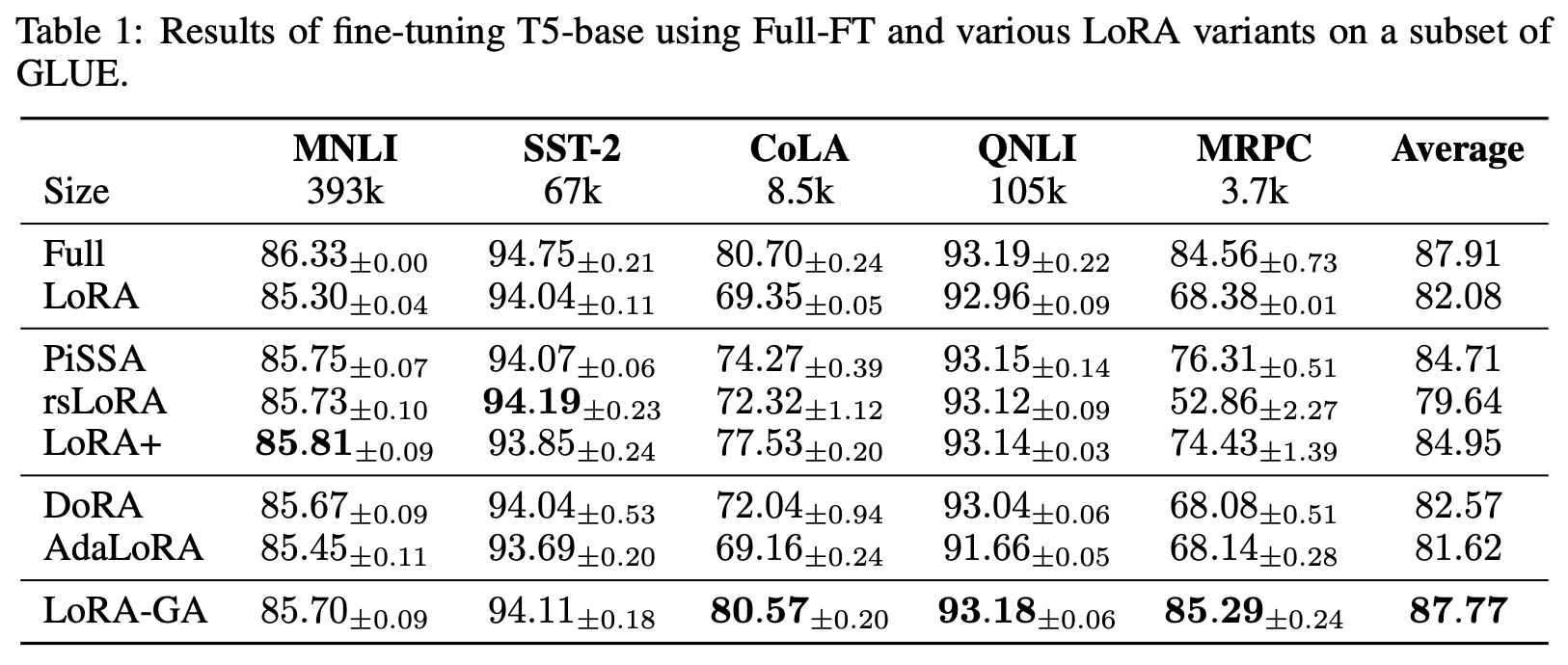 LoRA-GA + T5-Base performance on GLUE
On average, the smaller the amount of training data, the larger the relative improvement — which suggests that LoRA-GA's strategy of aligning with full fine-tuning not only helps improve the final results but also improves training efficiency, i.e., it can achieve better results with fewer training steps.
Its performance on LLAMA2-7b is also noteworthy:
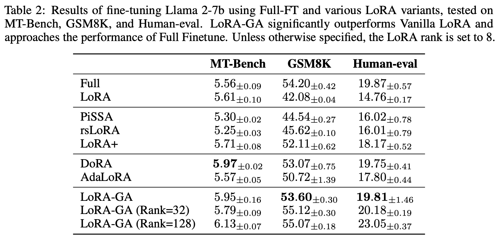 LoRA-GA + LLAMA2-7b performance on several benchmarks
Note that the main scenario in which LoRA is used is when GPU memory is insufficient, but LoRA's initialization requires computing the full gradient for all trainable parameters, which itself may be infeasible due to insufficient memory. To address this, the trick proposed in the original paper is to compute gradients for parameters one at a time in a serial fashion, rather than computing gradients for all trainable parameters simultaneously — this reduces the memory needed for each individual computation step. Serial gradient computation does reduce efficiency, but since initialization itself is a one-time task, being a bit slower is not a problem. As for how to implement this in practice, different frameworks have different approaches, which we won't go into here.
Summary
This post has introduced LoRA-GA, a new improvement to LoRA. Although various LoRA variants are hardly rare, LoRA-GA won me over with its remarkably intuitive theoretical guidance — its line of reasoning gives one the feeling of "I've looked into its eyes, and this is the right paper." Combined with its noteworthy experimental results, the whole thing flows as smoothly as water, a genuine pleasure to read.
Translated automatically with claude-sonnet-5; all equations are reproduced verbatim from the source. Copyright remains with the original author.