Aligning with Full Fine-tuning! The Most Brilliant LoRA Improvement I've Seen (Part 2)
Two weeks ago I wrote Aligning with Full Fine-tuning! The Most Brilliant LoRA I've Seen (Part 1) (which wasn't numbered "Part 1" at the time), introducing a LoRA variant called "LoRA-GA," which improves LoRA's initialization via a gradient SVD, thereby aligning LoRA with full fine-tuning. Of course, theoretically speaking, this can only align $W_1$ after the first update step as closely as possible, so at the time some readers raised the question "what about $W_2,W_3,\cdots$ afterward — are those just ignored?" I hadn't thought too deeply about it back then, and simply felt that once the first step was aligned, subsequent optimization would follow a reasonably good trajectory as well.
Interestingly, not long after LoRA-GA came out, a new paper appeared on arXiv, LoRA-Pro: Are Low-Rank Adapters Properly Optimized?, and the LoRA-Pro method it proposes answers exactly this question! LoRA-Pro likewise aims to align with full fine-tuning, but what it aligns is the gradient at every step, thereby aligning the entire optimization trajectory — which turns out to be exactly the complementary improvement to LoRA-GA.
Aligning with Full Fine-tuning
This post continues using the notation and content from the previous article, so here I'll just briefly recap the previous section's content rather than repeating it in detail. LoRA's parameterization is
\begin{equation}W = (W_0 - A_0 B_0) + AB\end{equation}more
where $W_0 \in \mathbb{R}^{n\times m}$ is the pretrained weight, $A\in\mathbb{R}^{n\times r},B\in\mathbb{R}^{r\times m}$ are the newly introduced trainable parameters, and $A_0,B_0$ are their initial values.
In the previous section we noted that full fine-tuning often outperforms LoRA, so full fine-tuning is exactly the direction LoRA should most try to align with. To quantify this, we can write out the SGD update formulas for full fine-tuning and LoRA fine-tuning respectively, giving
\begin{equation} W_{t+1} = W_t - \eta G_t\end{equation}
and
\begin{equation}\begin{gathered} A_{t+1} = A_t - \eta G_{A,t} = A_t - \eta G_t B_t^{\top},\quad B_{t+1} = B_t - \eta G_{B,t} = B_t - \eta A_t^{\top}G_t \\[8pt] W_{t+1} = W_t - A_t B_t + A_{t+1} B_{t+1} \approx W_t - \eta(A_t A_t^{\top}G_t + G_tB_t^{\top} B_t) \end{gathered}\end{equation}
where $\mathcal{L}$ is the loss function, $\eta$ is the learning rate, and we also have $G_t=\frac{\partial \mathcal{L}}{\partial W_t}$, $G_{A,t}=\frac{\partial \mathcal{L}}{\partial A_t}=\frac{\partial \mathcal{L}}{\partial W_t} B_t^{\top}=G_t B_t^{\top}$, and $G_{B,t}=\frac{\partial \mathcal{L}}{\partial B_t}=A_t^{\top}\frac{\partial \mathcal{L}}{\partial W_t} =A_t^{\top}G_t$.
LoRA-GA's idea is that we should at least make the $W_1$ of full fine-tuning and LoRA as close as possible, so it minimizes the objective
\begin{equation}\mathop{\text{argmin}}_{A_0,B_0}\left\Vert A_0 A_0^{\top}G_0 + G_0 B_0^{\top} B_0 - G_0\right\Vert_F^2\end{equation}
whose optimal solution can be obtained via SVD of $G_0$, from which we can find the optimal $A_0,B_0$ to use as the initialization for $A,B$.
Step-by-Step Alignment
LoRA-Pro's idea goes further: it wants to align every single $W_t$ of full fine-tuning and LoRA, not just the first one. But how can this be achieved? Should we minimize $\left\Vert A_t A_t^{\top}G_t + G_t B_t^{\top} B_t - G_t\right\Vert_F^2$ at every step? That's clearly not right, because $A_t,B_t$ is determined by the optimizer based on $A_{t-1},B_{t-1}$ and their gradients — it's not a freely adjustable parameter.
It might seem there's nothing left for us to modify. But no — LoRA-Pro cleverly realizes: since "$A_t,B_t$ is determined by the optimizer based on $A_{t-1},B_{t-1}$ and their gradients," and we can't change $A_{t-1},B_{t-1}$ or the gradients themselves, we can still change the optimizer! Specifically, we modify the update rule for $A_t,B_t$ to:
\begin{equation}\begin{gathered} A_{t+1} = A_t - \eta H_{A,t} \\ B_{t+1} = B_t - \eta H_{B,t} \end{gathered}\end{equation}
where $H_{A,t},H_{B,t}$ are yet to be determined, but their shapes match $A,B$. We can now write
\begin{equation}W_{t+1} = W_t - A_t B_t + A_{t+1} B_{t+1} \approx W_t - \eta(H_{A,t} B_t + A_t H_{B,t}) \end{equation}
At this point we can tune $H_{A,t},H_{B,t}$ so that this $W_{t+1}$ is as close as possible to SGD's $W_{t+1}$:
\begin{equation}\mathop{\text{argmin}}_{H_{A,t},H_{B,t}}\left\Vert H_{A,t} B_t + A_t H_{B,t} - G_t\right\Vert_F^2\end{equation}
Let's now solve this optimization problem. For simplicity, during the derivation we'll drop the subscript $t$, i.e., consider
\begin{equation}\mathop{\text{argmin}}_{H_A,H_B}\left\Vert H_A B + A H_B - G\right\Vert_F^2\label{eq:loss}\end{equation}
Simplifying the Objective
Since there's no constraint between $H_A,H_B$, the optimization over $H_A,H_B$ is independent, so we can adopt the strategy of first optimizing $H_A$ and then $H_B$ (or the reverse order works too). When optimizing $H_A$, $H_B$ is treated as a constant, so let's first consider the following simplified equivalent problem
\begin{equation}\mathop{\text{argmin}}_H\left\Vert H B - X\right\Vert_F^2\label{eq:h-xb-loss}\end{equation}
where $H\in\mathbb{R}^{n\times r},B\in\mathbb{R}^{r\times m},X\in\mathbb{R}^{n\times m}$. If $r=m$ and $B$ is invertible, we can directly reduce this to solving the linear system $HB=X$, i.e., $H=XB^{-1}$. When $r < m$, we need to resort to optimization tools; noting that $HB-X$ is linear in $H$, this is essentially a least-squares linear regression problem, which has an analytical solution:
\begin{equation}H = XB^{\top}(B B^{\top})^{-1} \label{eq:h-xb}\end{equation}
where $B^{\top}(B B^{\top})^{-1}$ is exactly the "pseudo-inverse" of the matrix $B$. If you're not familiar with this result, no worries — let's derive it directly. First, denote $\mathcal{l}=\left\Vert H B - X\right\Vert_F^2$, and take the derivative of $H$ directly to get
\begin{equation}\frac{\partial l}{\partial H} = 2(HB - X)B^{\top} = 2(HBB^{\top} - XB^{\top})\end{equation}
Then setting this equal to zero gives us $\eqref{eq:h-xb}$. For readers not so familiar with the rules of matrix differentiation: by the chain rule, it's not hard to see that $\frac{\partial l}{\partial H}$ must be $2(HB - X)$ and $B$ multiplied together in some way; and if we agree that $\frac{\partial l}{\partial H}$ has the same shape as $H$, i.e., $n\times r$, then the only way to combine $2(HB - X)$ and $B$ into a result of shape $n\times r$ is $2(HB - X)B^{\top}$.
Similarly, the derivative of $\left\Vert AH - X\right\Vert_F^2$ with respect to $H$ is $2A^{\top}(AH - X)$, from which we obtain
\begin{equation}\mathop{\text{argmin}}_H\left\Vert AH - X\right\Vert_F^2\quad\Rightarrow\quad H = (A^{\top} A)^{-1}A^{\top}X \label{eq:h-ax}\end{equation}
The Complete Result
With the results $\eqref{eq:h-xb}$ and $\eqref{eq:h-ax}$ in hand, we can proceed to solve $\eqref{eq:loss}$. First we fix $H_B$, so that according to equation $\eqref{eq:h-xb}$ we get
\begin{equation}H_A = (G - A H_B) B^{\top}(B B^{\top})^{-1}\label{eq:h-a-1}\end{equation}
Notice that the objective function in equation $\eqref{eq:loss}$ has an invariance:
\begin{equation}\left\Vert H_A B + A H_B - G\right\Vert_F^2 = \left\Vert (H_A + AC) B + A (H_B - CB) - G\right\Vert_F^2\end{equation}
where $C$ is any matrix of shape $r\times r$. That is, the solution for $H_A$ can have any matrix of the form $AC$ added or subtracted, as long as $H_B$ has the corresponding $CB$ subtracted or added. Using this property, we can simplify the $H_A$ in equation $\eqref{eq:h-a-1}$ to
\begin{equation}H_A = G B^{\top}(B B^{\top})^{-1}\end{equation}
Substituting back into the objective function gives
\begin{equation}\mathop{\text{argmin}}_{H_B}\left\Vert A H_B - G(I - B^{\top}(B B^{\top})^{-1}B)\right\Vert_F^2\end{equation}
According to equation $\eqref{eq:h-ax}$ we get
\begin{equation}H_B = (A^{\top} A)^{-1}A^{\top}G(I - B^{\top}(B B^{\top})^{-1}B)\end{equation}
Noting that $G B^{\top},A^{\top}G$ are exactly the gradients $G_A,G_B$ of $A,B$, and by once again applying the invariance mentioned above, we can write down the complete solution
\begin{equation}\left\{\begin{aligned} H_A =&\, G_A (B B^{\top})^{-1} + AC \\ H_B =&\, (A^{\top} A)^{-1}G_B(I - B^{\top}(B B^{\top})^{-1}B) - CB \end{aligned}\right.\end{equation}
The Optimal Parameter
At this point we've solved for the form of $H_A,H_B$, but the solution isn't unique — it has a freely-chosen parameter matrix $C$. We can choose an appropriate $C$ so that the resulting $H_A,H_B$ has some desired properties.
For instance, currently $H_A,H_B$ is not very symmetric, since $H_B$ has the extra term $-(A^{\top} A)^{-1}G_B B^{\top}(B B^{\top})^{-1}B$; we can distribute this evenly across $H_A,H_B$ to make things more symmetric, which corresponds to choosing $C = -\frac{1}{2}(A^{\top} A)^{-1}G_B B^{\top}(B B^{\top})^{-1}$ as:
\begin{equation}\left\{\begin{aligned} H_A =&\, \left[I - \frac{1}{2}A(A^{\top}A)^{-1}A^{\top}\right]G_A (B B^{\top})^{-1} \\ H_B =&\, (A^{\top} A)^{-1}G_B\left[I - \frac{1}{2}B^{\top}(B B^{\top})^{-1}B\right] \end{aligned}\right.\end{equation}
This $C$ is also the solution to the following two optimization problems:
\begin{align} &\,\mathop{\text{argmin}}_C \Vert H_A B - A H_B\Vert_F^2 \\ &\,\mathop{\text{argmin}}_C \Vert H_A B - G\Vert_F^2 + \Vert A H_B - G\Vert_F^2 \\ \end{align}
The first optimization objective can be understood as making the contributions of $A,B$ to the final result as equal as possible, which shares some kinship with the assumption in Configuring Different Learning Rates — Can LoRA Do Even Better?; the second optimization objective is about making both $H_A B$ and $A H_B$ as close as possible to the full gradient $G$. Taking $l=\Vert H_A B - A H_B\Vert_F^2$ as an example, differentiating directly gives
\begin{equation}\frac{\partial l}{\partial C} = 4A^{\top}(H_A B - A H_B)B^{\top}=4A^{\top}\left[G_A (BB^{\top})^{-1}B + 2ACB\right]B^{\top}\end{equation}
Setting this equal to zero, we can solve for the same $C$; the key steps in the simplification are $[I - B^{\top}(B B^{\top})^{-1}B]B^{\top} = 0$ and $A^{\top}G_A = G_B B^{\top}$.
The $C$ chosen by LoRA-Pro is slightly different — it's the optimal solution of the following objective function:
\begin{equation}\mathop{\text{argmin}}_C \Vert H_A - G_A\Vert_F^2 + \Vert H_B - G_B\Vert_F^2\end{equation}
The intent here is also clear: since $H_A,H_B$ is meant to replace $G_A,G_B$, it's a reasonable choice to keep the change from $G_A,G_B$ as small as possible while achieving the same effect. Again taking the derivative with respect to $C$ and setting it to zero, after simplification we get
\begin{equation}A^{\top}A C + C B B^{\top} = -A^{\top} G_A (BB^{\top})^{-1}\end{equation}
We now have an equation in $C$; this type of equation is called a "Sylvester equation," and its analytical solution for $C$ can be written using outer-product notation, but there's no real need to, since solving it numerically directly is actually cheaper than the analytical solution — so we just solve it numerically. Overall, these various choices for $C$ are all about making $H_A,H_B$ more symmetric from some perspective; although I haven't personally run comparison experiments, I don't think there's likely to be a very noticeable difference between these different choices.
General Discussion
Let's recap what we've derived so far. Our model is still ordinary LoRA, and the goal is to have every update step approximate the result of full fine-tuning. To this end, we assumed the optimizer is SGD, and then compared the $W_{t+1}$ obtained by full fine-tuning and LoRA under the same $W_t$, finding that to achieve this goal, the gradient $G_A, G_B$ used to update $A,B$ needs to be replaced with the $H_A,H_B$ derived above.
Next we return to the familiar issue in optimization analysis: the preceding analysis was all based on the SGD optimizer, but in practice we more commonly use Adam — so how should things change there? If we repeat the previous derivation for the Adam optimizer, the result is that the gradient $G$ in $H_A,H_B$ needs to be replaced with Adam's update direction $U$ under full fine-tuning. However, $U$ needs to be computed from the full fine-tuning gradient $G$ using Adam's update rule, and since our setting is LoRA, we have no access to the full fine-tuning gradient — only the gradient $G_A,G_B$ of $A,B$.
Nevertheless, we can consider an approximate scheme: since the optimization objective of $H_A B + A H_B$ mentioned earlier is precisely to approximate $G$, we can use it as an approximation to $G$ when running Adam, and this way the whole pipeline works out. So we can write the following update rule
\begin{equation}\begin{array}{l} \begin{array}{l}G_A = \frac{\partial\mathcal{L}}{\partial A_{t-1}},\,\,G_B = \frac{\partial\mathcal{L}}{\partial B_{t-1}}\end{array} \\ \color{green}{\left.\begin{array}{l}H_A = G_A (B B^{\top})^{-1} \\ H_B = (A^{\top} A)^{-1}G_B(I - B^{\top}(B B^{\top})^{-1}B) \\ \tilde{G} = H_A B + A H_B \end{array}\quad\right\} \text{estimated gradient}} \\ \color{red}{\left.\begin{array}{l}M_t = \beta_1 M_{t-1} + (1 - \beta_1) \tilde{G} \\ V_t = \beta_2 V_{t-1} + (1 - \beta_2) \tilde{G}^2 \\ \hat{M}_t = \frac{M_t}{1-\beta_1^t},\,\,\hat{V}_t = \frac{V_t}{1-\beta_2^t},\,\,U = \frac{\hat{M}_t}{\sqrt{\hat{V}_t + \epsilon}}\end{array}\quad\right\} \text{Adam update}} \\ \color{purple}{\left.\begin{array}{l}U_A = UB^{\top},\,\, U_B = A^{\top} U \\ \tilde{H}_A = U_A (B B^{\top})^{-1} + AC \\ \tilde{H}_B = (A^{\top} A)^{-1}U_B(I - B^{\top}(B B^{\top})^{-1}B) - CB \end{array}\quad\right\} \text{project to}A,B} \\ \begin{array}{l}A_t = A_{t-1} - \eta \tilde{H}_A \\ B_t = B_{t-1} - \eta \tilde{H}_B \\ \end{array} \\ \end{array}\end{equation}
This is also the update algorithm ultimately used by LoRA-Pro (more precisely, LoRA-Pro uses AdamW, which is slightly more complex, but not substantively different). However, setting aside the extra complexity this modification introduces, the biggest issue with this algorithm is that the moving-average update variable $M,V$ inside it, just like in full fine-tuning, is full-rank — meaning its optimizer doesn't actually save GPU memory compared to full fine-tuning; it only saves some memory on parameters and gradients via low-rank decomposition. This still represents a noticeable increase in memory usage compared to ordinary LoRA.
A relatively simple scheme (though I haven't tested it) would be to directly substitute $H_A,H_B$ for $G_A,G_B$ and then compute using the ordinary LoRA Adam update rule, so that the shape of $M,V$ matches the corresponding $A,B$, maximizing the memory savings. But the theoretical justification for Adam in this case is weaker than LoRA-Pro's version of Adam, relying more, as in Aligning with Full Fine-tuning! The Most Brilliant LoRA I've Seen (Part 1), on faith that "conclusions from SGD can be applied in parallel to Adam."
Experimental Results
LoRA-Pro's experimental results on GLUE are even more impressive, surpassing the results of full fine-tuning:
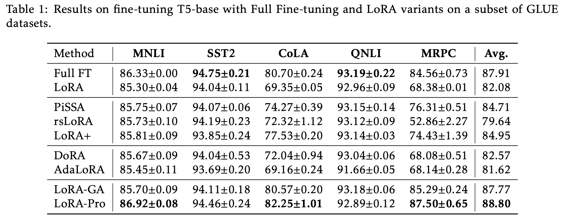 LoRA-Pro's experimental results on GLUE
However, the paper contains only this one experiment. It seems LoRA-Pro was written up rather hastily — perhaps upon seeing LoRA-GA, the authors felt the overlap was too obvious and rushed to stake their claim first. My first reaction upon skimming LoRA-Pro was also that it overlapped with LoRA-GA, but on closer reading I found that the two are actually complementary results under the same underlying idea.
Looking at LoRA-Pro's result, it involves inverting $A^{\top} A$ and $B B^{\top}$, so it's clear that one of $A,B$ can no longer be initialized to all zeros — the more intuitively fitting choice is orthogonal initialization, i.e., making the initial $A^{\top} A,B B^{\top}$ a (scaled) identity matrix. And as it happens, from Aligning with Full Fine-tuning! The Most Brilliant LoRA I've Seen (Part 1) we can see that the initialization given by LoRA-GA is precisely an orthogonal initialization — so LoRA-Pro and LoRA-GA turn out to be the "perfect pairing."
Summary
This post introduced another piece of work aligning with full fine-tuning, LoRA-Pro, which turns out to be complementary to the LoRA-GA discussed in the previous post. LoRA-GA tries to align LoRA with full fine-tuning by improving the initialization, while LoRA-Pro goes further, modifying the optimizer's update rule so that every single update step of LoRA aligns as closely as possible with full fine-tuning. Both are brilliant LoRA improvements, and both are genuinely delightful pieces of work.
Translated automatically with claude-sonnet-5; all equations are reproduced verbatim from the source. Copyright remains with the original author.