A Brief Look at the "Curse of Dimensionality": The Hubness Phenomenon

“维度灾难”之Hubness现象浅析 苏剑林 · 2022-06-28 · Machine Learning dimension GAN generative model

A few days ago I came across the paper Exploring and Exploiting Hubness Priors for High-Quality GAN Latent Sampling, and through it I learned a new term: the "Hubness phenomenon." It describes a kind of clustering effect in high-dimensional space, which is fundamentally one of the many manifestations of the "curse of dimensionality." The paper uses the concept of hubness to derive a scheme for improving the generation quality of GAN models, which struck me as quite interesting. So I went ahead and looked into the Hubness phenomenon a bit, and I'm recording what I learned here for reference.

The collapsing ball

The "curse of dimensionality" is a rather broad concept — any conclusion that, in high dimensions, deviates drastically from its two- or three-dimensional counterpart can be called an instance of the curse of dimensionality. For example, in The Angle Distribution Between Two Random Vectors in n-Dimensional Space we introduced the fact that "in high-dimensional space, almost any two vectors are nearly orthogonal." Quite a few of these curse-of-dimensionality phenomena actually share a common origin — namely, that "the ratio of the volume of a unit ball in high-dimensional space to that of its circumscribing cube collapses to 0" — and the subject of this post, the Hubness phenomenon, is no exception.more

In A Masterstroke: Computing the Volume of an n-Dimensional Ball, we derived the volume formula for an $n$-dimensional ball, from which we know that the volume of an $n$-dimensional unit ball is

\begin{equation}V_n = \frac{\pi^{n/2}}{\Gamma\left(\frac{n}{2}+1\right)}\end{equation}

The corresponding circumscribing cube has side length $2$, so its volume is naturally $2^n$, and the corresponding volume ratio is $V_n / 2^n$. Its graph looks like this:

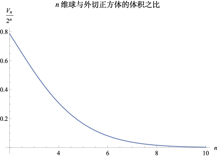Ratio of the volume of an n-dimensional ball to its circumscribing cube

As we can see, as the dimension grows, this ratio quickly tends to 0. A vivid way of putting this conclusion is: "as dimension increases, the ball becomes more and more negligible." It tells us that if we try to achieve uniform sampling inside a ball via "uniform distribution + rejection sampling," the efficiency will be extremely low in high-dimensional space (the rejection rate approaches 100%). Another way to understand it is that "most of the points inside a high-dimensional ball are concentrated near its surface," and the proportion of the region near the center of the ball becomes ever smaller.

The Hubness phenomenon

Now let's turn to the Hubness phenomenon. It describes the following situation: if we randomly pick a batch of points in high-dimensional space, "there are always some points that keep showing up among the $k$-nearest neighbors of other points."

How should we understand this statement concretely? Suppose we have $N$ points $x_1,x_2,\cdots,x_N$. For each $x_i$, we can find its $k$ closest points, and these $k$ points are called the "$k$-nearest neighbors of $x_i$." With the concept of $k$-nearest neighbors in hand, we can count, for each point, how many times it appears among the $k$-nearest neighbors of other points; this count is called the "hub value." The larger a point's hub value, the more likely it is to show up in the $k$-nearest neighbors of other points.

So, the Hubness phenomenon says: there are always a handful of points whose hub values are conspicuously large. If we think of the hub value as representing "wealth," a vivid analogy would be "80% of the wealth is concentrated in the hands of 20% of the people" — and as the dimension increases, this "wealth gap" only grows larger. If instead we think of the hub value as representing "social connections," then a fitting analogy would be "in any community there are always a few people with an extraordinarily broad network of connections."

How does the Hubness phenomenon arise? It is actually related to the collapse of the $n$-dimensional ball discussed in the previous section. We know that the point minimizing the sum of squared distances to all other points is exactly the mean point:

\begin{equation}\frac{1}{N} \sum_{i=1}^N x_i = c^* = \mathop{\text{argmin}}_c \sum_{i=1}^N \Vert x_i - c\Vert^2\end{equation}

This means that points near the mean vector have, on average, smaller distances to all other points, and thus have a greater chance of becoming the $k$-nearest neighbor of many points. Meanwhile, the collapse phenomenon of the $n$-dimensional ball tells us that "the region near the mean vector" — i.e., a ball-shaped neighborhood centered at the mean vector — occupies a vanishingly small proportion of the space. Hence we get the phenomenon that "a very small number of points show up among the $k$-nearest neighbors of many points." Of course, using the mean vector here is just an intuitive way of putting it; for general data points, it should be that the closer a point is to the density center, the larger its hub value tends to become.

Improving sampling

So what does the scheme for improving GAN generation quality mentioned at the start of this post have to do with the Hubness phenomenon? The paper Exploring and Exploiting Hubness Priors for High-Quality GAN Latent Sampling proposes a prior hypothesis: the larger the hub value, the better the generation quality of the corresponding point.

Specifically, the typical GAN sampling-and-generation pipeline is $z\sim \mathcal{N}(0,1), x=G(z)$. We can first sample $N$ sample points $z_1,z_2,\cdots,z_N$ from $\mathcal{N}(0,1)$, and then compute the hub value for each sample point. The original paper found that the hub value is positively correlated with generation quality, so they keep only the sample points whose hub value is greater than or equal to a threshold $t$ to use for generation. This is a "pre-hoc" filtering approach; reference code is as follows:

def get_z_samples(size, t=50):
    """通过Hub值对采样结果进行筛选
    """
    Z = np.empty((0, z_dim))
    while len(Z) < size:
        z = np.random.randn(10000, z_dim)
        s = np.zeros(10000)
        for i in range(10):
            zi = z[i * 1000:(i + 1) * 1000]
            d = (z**2).sum(1)[:, None] + (zi**2).sum(1)[None] - 2 * z.dot(zi.T)
            for j in d.argsort(0)[1:1 + 5].T:
                s[j] += 1
        z = z[s > t]
        Z = np.concatenate([Z, z], 0)[:size]
        print('%s / %s' % (len(Z), size))
    return Z

Why does filtering by hub value work? From the discussion above, we know that the larger the hub value, the closer the point is to the center of the sample — or, more precisely, the closer it is to the density center — which means it has many neighboring points around it. That makes it unlikely to be an under-trained outlier, and hence the resulting generation quality tends to be relatively higher. Multiple experiments in the paper confirm this conclusion.

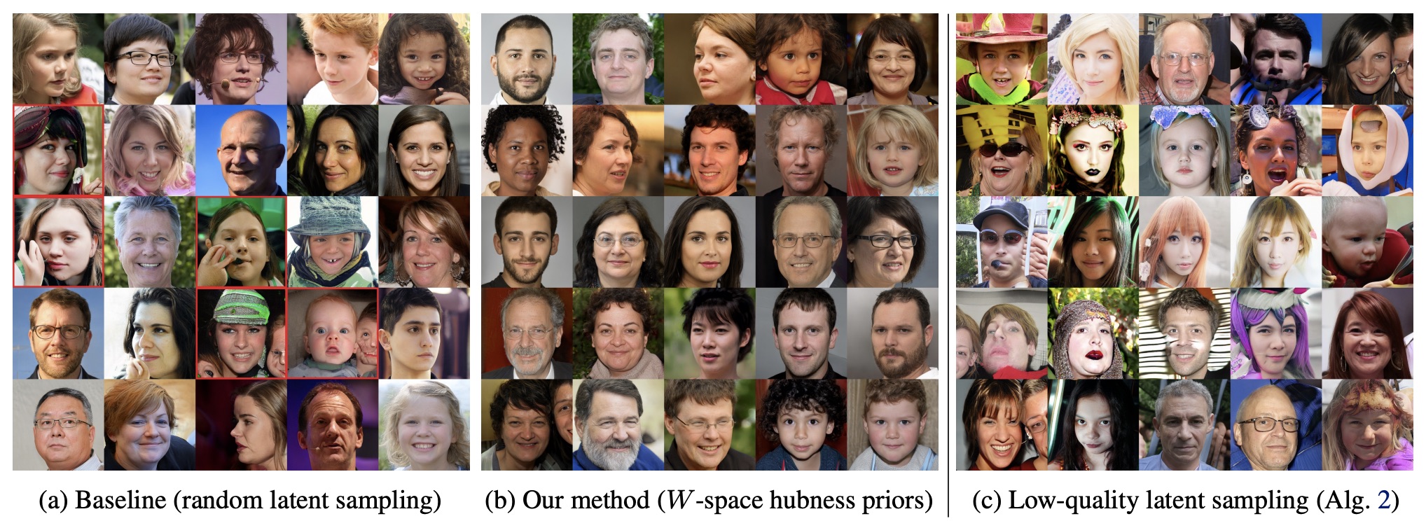Comparison of generation quality when filtering based on hub value

Summary

This post gave a brief introduction to the Hubness phenomenon, one manifestation of the "curse of dimensionality," and described its application in improving the generation quality of GANs.