CAN: A Simple Post-Processing Trick to Boost Classification Performance via Prior Distributions

CAN：借助先验分布提升分类性能的简单后处理技巧 苏剑林 · 2021-10-22 · Machine Learning model probability analysis technique

As the name suggests, this post introduces a post-processing trick for classification problems called CAN (Classification with Alternating Normalization), from the paper When in Doubt: Improving Classification Performance with Alternating Normalization. Having tested it myself, I've found that CAN does improve the performance of multi-class classification in most cases, and it adds almost no extra inference cost, since it's simply a lightweight re-normalization of the prediction results.

Interestingly, the idea behind CAN is actually very simple—so simple that everyone has probably applied the same intuition in everyday life. Yet the CAN paper doesn't explain this idea very clearly; it presents and evaluates the method in a purely formal way. In this post, I'll try to make the underlying idea as clear as possible.

An Illustrative Example

Suppose we have a binary classification problem, and for input $a$ the model gives a prediction of $p^{(a)} = [0.05, 0.95]$; then we can confidently assign it to class $1$. Next, for input $b$, the model gives a prediction of $p^{(b)}=[0.5,0.5]$—at this point we're in the most uncertain state possible, with no clue which class to pick. more

But suppose I tell you two things: 1) the label must be either 0 or 1; 2) each class occurs with probability 0.5 in general. Given this prior information, since the previous sample was predicted as class 1, wouldn't it make sense—following a naive "balance" intuition—to lean toward predicting the second sample as class 0, so that the overall predictions better match the second prior?

There are many examples like this. Say you're doing 10 multiple-choice questions: you're fairly confident about the first 9, but have no idea about the 10th and just have to guess. Then you notice that among your answers to the first 9 questions, you picked A, B, and C, but never D. Wouldn't you then be more inclined to guess D for the 10th question?

Behind these simple examples lies the same idea as CAN: it uses a prior distribution to correct low-confidence predictions, so that the distribution of the new predictions moves closer to the prior distribution.

Uncertainty

To be precise, CAN is a post-processing method targeted at low-confidence predictions, so we first need a metric to quantify the uncertainty of a prediction. A common choice is "entropy" (see Entropy Unravelled: From Entropy and the Maximum Entropy Principle to Maximum Entropy Models (Part 1)); for $p=[p_1,p_2,\cdots,p_m]$, it is defined as:

\begin{equation}H(p) = -\sum_{i=1}^m p_i\log p_i\end{equation}

However, although entropy is a common choice, the results it gives don't always match our intuition. For instance, for $p^{(a)}=[0.5,0.25,0.25]$ and $p^{(b)}=[0.5,0.5,0]$, plugging directly into the formula gives $H(p^{(a)}) > H(p^{(b)})$, but in our classification setting, we'd clearly consider $p^{(b)}$ to be more uncertain than $p^{(a)}$. So using entropy directly isn't quite reasonable.

A simple fix is to compute the entropy using only the top-$k$ probability values. Without loss of generality, suppose $p_1,p_2,\cdots,p_k$ are the $k$ largest probability values; then

\begin{equation}H_{\text{top-}k}(p) = -\sum_{i=1}^k \tilde{p}_i\log \tilde{p}_i\end{equation}

where $\tilde{p}_i=p_i\Big/ \sum\limits_{i=1}^k p_i$. To get a result in the range 0–1, we take $H_{\text{top-}k}(p)/\log k$ as the final uncertainty metric.

Algorithm Steps

Now suppose we have $N$ samples to classify, and the model's direct predictions are $N$ probability distributions $p^{(1)},p^{(2)},\cdots,p^{(N)}$. Assuming the test samples and training samples are drawn from the same distribution, a perfect set of predictions should satisfy:

\begin{equation}\frac{1}{N}\sum_{i=1}^N p^{(i)} = \tilde{p}\label{eq:prior}\end{equation}

where $\tilde{p}$ is the prior distribution over classes, which we can estimate directly from the training set. In other words, the overall predictions should be consistent with the prior distribution, but due to limitations in model performance and other factors, the actual predictions may deviate noticeably from the equation above. This is exactly the part we can correct manually.

Specifically, we choose a threshold $\tau$, treating predictions with a metric value smaller than $\tau$ as high-confidence, and those greater than or equal to $\tau$ as low-confidence. Without loss of generality, assume the first $n$ results $p^{(1)},p^{(2)},\cdots,p^{(n)}$ are high-confidence, and the remaining $N-n$ are low-confidence. We treat the high-confidence subset as more reliable, so it doesn't need correcting, and we can use it as a "reference frame" to correct the low-confidence subset.

Specifically, for $\forall j\in\{n+1,n+2,\cdots,N\}$, we take $p^{(j)}$ together with the high-confidence set $p^{(1)},p^{(2)},\cdots,p^{(n)}$ and perform one round of "row-wise" normalization:

\begin{equation}p^{(k)} \leftarrow p^{(k)}\big/\bar{p}\times\tilde{p},\quad\bar{p}=\frac{1}{n+1}\left(p^{(j)} + \sum_{i=1}^n p^{(i)}\right)\label{eq:step-1}\end{equation}

Here $k\in\{1,2,\cdots,n\}\cup\{j\}$, where the multiplication and division are element-wise. It's not hard to see that the purpose of this normalization step is to make the average vector of all the new $p^{(k)}$'s equal to the prior distribution $\tilde{p}$, i.e., to enforce equation $\eqref{eq:prior}$. However, after this normalization, each $p^{(k)}$ may no longer sum to 1, so we also need a "column-wise" normalization step:

\begin{equation}p^{(k)} \leftarrow \frac{p^{(k)}_i}{\sum\limits_{i=1}^m p^{(k)}_i}\label{eq:step-2}\end{equation}

But then equation $\eqref{eq:prior}$ might no longer hold. So in theory we could alternate between these two steps repeatedly until convergence (although experiments show that a single iteration usually works best). Finally, we keep only the updated $p^{(j)}$ as the prediction for the original $j$-th sample, discarding the rest of the $p^{(k)}$ values.

Note that this process must be applied by looping over each low-confidence result $j\in\{n+1,n+2,\cdots,N\}$ individually—that is, corrections are made sample by sample rather than all at once. Each $p^{(j)}$ is combined with the original high-confidence results $p^{(1)},p^{(2)},\cdots,p^{(n)}$ and iterated through the steps above. Although during iteration the corresponding $p^{(1)},p^{(2)},\cdots,p^{(n)}$ get updated, those are just temporary results that are ultimately discarded—each correction always uses the original $p^{(1)},p^{(2)},\cdots,p^{(n)}$.

Reference Implementation

Here's a reference implementation:

# 预测结果，计算修正前准确率
y_pred = model.predict(
    valid_generator.fortest(), steps=len(valid_generator), verbose=True
)
y_true = np.array([d[1] for d in valid_data])
acc_original = np.mean([y_pred.argmax(1) == y_true])
print('original acc: %s' % acc_original)

# 评价每个预测结果的不确定性
k = 3
y_pred_topk = np.sort(y_pred, axis=1)[:, -k:]
y_pred_topk /= y_pred_topk.sum(axis=1, keepdims=True)
y_pred_uncertainty = -(y_pred_topk * np.log(y_pred_topk)).sum(1) / np.log(k)

# 选择阈值，划分高、低置信度两部分
threshold = 0.9
y_pred_confident = y_pred[y_pred_uncertainty < threshold]
y_pred_unconfident = y_pred[y_pred_uncertainty >= threshold]
y_true_confident = y_true[y_pred_uncertainty < threshold]
y_true_unconfident = y_true[y_pred_uncertainty >= threshold]

# 显示两部分各自的准确率
# 一般而言，高置信度集准确率会远高于低置信度的
acc_confident = (y_pred_confident.argmax(1) == y_true_confident).mean()
acc_unconfident = (y_pred_unconfident.argmax(1) == y_true_unconfident).mean()
print('confident acc: %s' % acc_confident)
print('unconfident acc: %s' % acc_unconfident)

# 从训练集统计先验分布
prior = np.zeros(num_classes)
for d in train_data:
    prior[d[1]] += 1.

prior /= prior.sum()

# 逐个修改低置信度样本，并重新评价准确率
right, alpha, iters = 0, 1, 1
for i, y in enumerate(y_pred_unconfident):
    Y = np.concatenate([y_pred_confident, y[None]], axis=0)
    for j in range(iters):
        Y = Y**alpha
        Y /= Y.mean(axis=0, keepdims=True)
        Y *= prior[None]
        Y /= Y.sum(axis=1, keepdims=True)
    y = Y[-1]
    if y.argmax() == y_true_unconfident[i]:
        right += 1

# 输出修正后的准确率
acc_final = (acc_confident * len(y_pred_confident) + right) / len(y_pred)
print('new unconfident acc: %s' % (right / (i + 1.)))
print('final acc: %s' % acc_final)

Experimental Results

So how much of a boost can this simple post-processing step actually deliver? The results reported in the original paper are quite impressive:

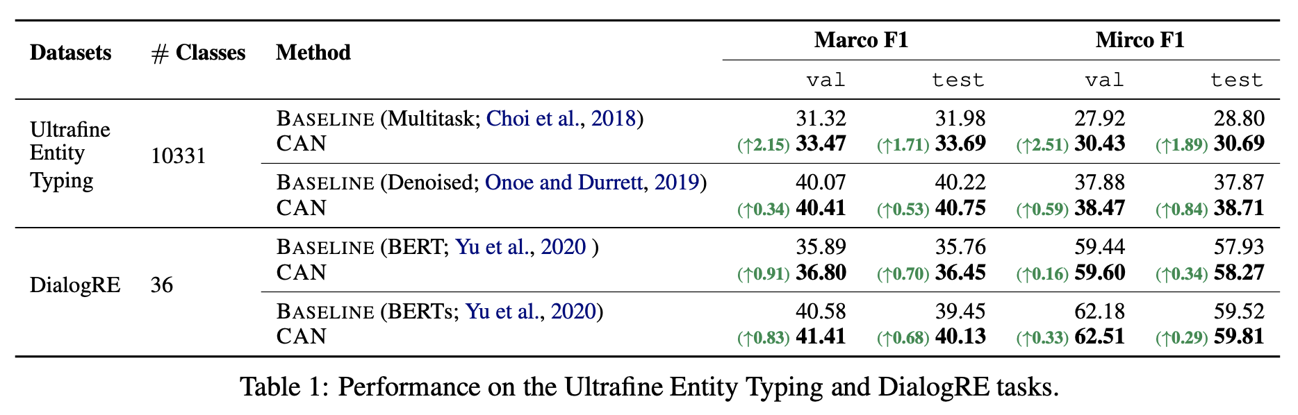One of the experimental results from the original paper

I also ran experiments on two Chinese text classification tasks from CLUE, and while there was some improvement, it was less dramatic (validation set results):

$$\begin{array}{c|c|c} \hline & \text{IFLYTEK (num classes: 119)} & \text{TNEWS (num classes: 15)}\\ \hline \text{BERT} & 60.06\% & 56.80\% \\ \text{BERT + CAN} & 60.52\% & 56.86\% \\ \hline \text{RoBERTa} & 60.64\% & 58.06\% \\ \text{RoBERTa + CAN} & 60.95\% & 58.00\% \\ \hline \end{array}$$

Generally speaking, the more classes there are, the more noticeable the improvement; if the number of classes is small, the improvement may be marginal or even slightly negative (though even the drops are minor), so this can be considered an "almost free lunch." As for hyperparameters, in the Chinese-language results above I ran only 1 iteration, with $k$ set to 3 and $\tau$ set to 0.9. After a bit of tuning, this turned out to be close to the optimal combination.

Some readers might wonder whether the earlier claim—that "the high-confidence subset is more reliable"—actually holds. At least in my two Chinese experiments, it clearly does. For example, in the IFLYTEK task, the accuracy on the filtered high-confidence set was 0.63+, while the low-confidence set only achieved 0.22+. The TNEWS task showed a similar pattern: 0.58+ accuracy on the high-confidence set versus only 0.23+ on the low-confidence set.

Personal Assessment

Let me wrap up with some overall thoughts and evaluation of CAN.

First, a natural question is: why not just lump all the low-confidence results together with the high-confidence ones and correct them in one batch, instead of correcting them one at a time? I don't know whether the original authors compared this, but I did test the idea myself, and the result was that batch correction sometimes matches individual correction, but sometimes performs worse. This actually makes sense: the whole point of CAN is to use the prior distribution together with the high-confidence results to correct the low-confidence ones. If we mix in too many low-confidence results at once, the resulting bias can grow larger. So in theory, correcting samples one by one should be more reliable than batch correction.

Speaking of the original paper, readers familiar with it may notice three differences between this post and the original CAN paper:

1. The uncertainty metric is computed differently. According to the original paper, the final uncertainty metric is computed as

\begin{equation}-\frac{1}{\log m}\sum_{i=1}^k p_i\log p_i\end{equation}

That is, it's also a top-$k$ entropy, but it doesn't renormalize these $k$ probability values, and the factor used to compress the result into the 0–1 range is $\log m$ rather than $\log k$ (since it isn't renormalized, only dividing by $\log m$ guarantees a value in 0–1). In my tests, the values computed this way in the original paper's formulation are usually noticeably below 1, which makes it harder to intuitively set and tune the threshold.

1. The presentation of CAN differs. The original paper describes the CAN algorithm in a purely mathematical, matrix-based way, without explaining where the idea comes from, which makes it fairly unfriendly for understanding. Without independently working through the underlying reasoning, it's hard to see why this kind of post-processing would improve classification performance at all—and once you do fully understand it, the original presentation can feel needlessly obscure.

1. The algorithm flow is slightly different. The original paper introduces an additional parameter $\alpha$ during iteration, turning equation $\eqref{eq:step-1}$ into

\begin{equation}p^{(k)} \leftarrow [p^{(k)}]^{\alpha}\big/\bar{p}\times\tilde{p},\quad\bar{p}=\frac{1}{n+1}\left([p^{(j)}]^{\alpha} + \sum_{i=1}^n [p^{(i)}]^{\alpha}\right)\end{equation}

That is, each result is raised to the power of $\alpha$ before the next iteration. Again, the original paper offers no explanation for this. In my view, this parameter is purely there to give more room for tuning (with more parameters, you can usually squeeze out some improvement somewhere), without much substantive meaning. In my own experiments, I found that $\alpha=1$ is essentially already the optimal choice, and fine-tuning $\alpha$ rarely yields any real benefit.

Summary

This post introduced a simple post-processing trick called CAN, which uses a prior distribution to renormalize prediction results, improving classification performance at almost no extra computational cost. Based on my experiments, CAN does deliver a measurable improvement in classification performance, and generally speaking, the more classes there are, the more pronounced the effect.