An orthogonal matrix that transforms one unit vector into another

从一个单位向量变换到另一个单位向量的正交矩阵 苏剑林 · 2021-06-05 · Mathematics transform vector matrix

In this post we discuss a fairly practical problem in linear algebra:

Given two $d$-dimensional unit (column) vectors $\boldsymbol{a},\boldsymbol{b}$, find an orthogonal matrix $\boldsymbol{T}$ such that $\boldsymbol{b}=\boldsymbol{T}\boldsymbol{a}$.

Since the two vectors have the same norm, it's clear that such an orthogonal matrix must exist. So how do we actually find it?

Two dimensions

It's not hard to imagine that this is essentially a problem of transforming vectors (say, by rotation or mirror reflection) within the two-dimensional subplane spanned by $\boldsymbol{a},\boldsymbol{b}$, so let's first consider the case $d=2$.

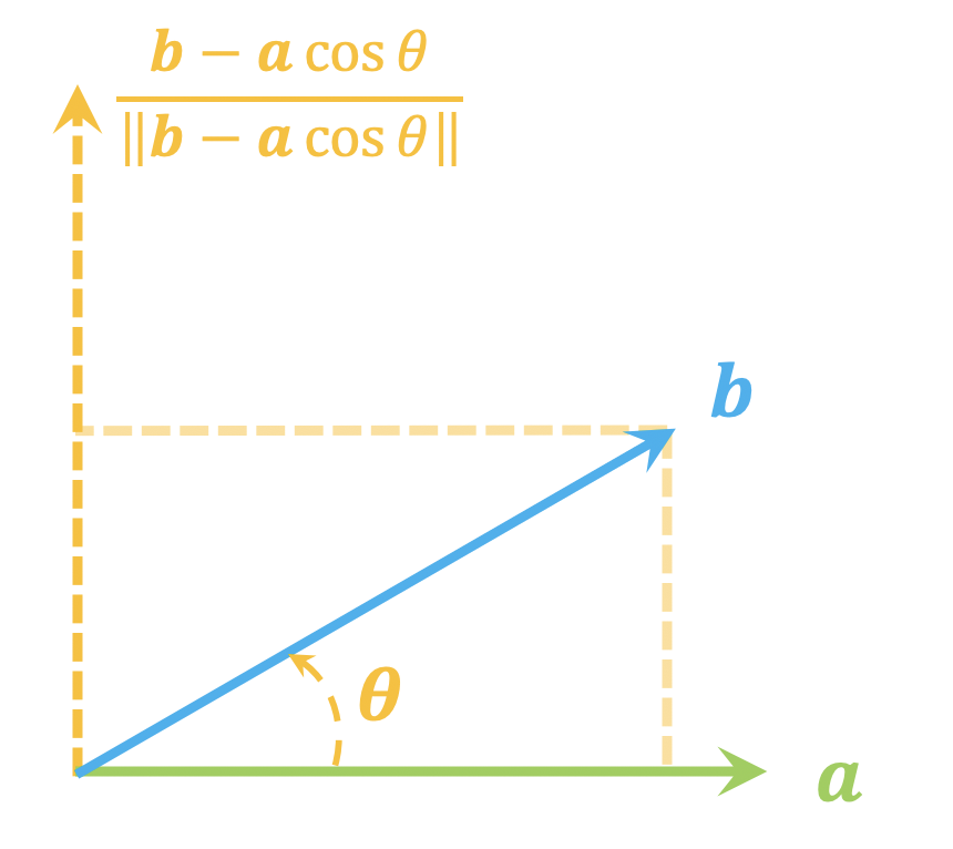Orthogonal decomposition diagram more

As shown in the figure above, through orthogonal decomposition we can obtain a vector $\boldsymbol{b} - \boldsymbol{a}\cos\theta$ perpendicular to $\boldsymbol{a}$, and after normalizing it we get an orthonormal basis:

\begin{equation}\boldsymbol{Q} = \begin{pmatrix}\boldsymbol{a} & \frac{\boldsymbol{b} - \boldsymbol{a}\cos\theta}{\Vert \boldsymbol{b} - \boldsymbol{a}\cos\theta\Vert}\end{pmatrix}\end{equation}

where $\theta$ is the angle between $\boldsymbol{a},\boldsymbol{b}$. Under this basis, the coordinates of $\boldsymbol{a}$ are $(1,0)$, and the coordinates of $\boldsymbol{b}$ are $(\cos\theta,\sin\theta)$, i.e.

\begin{equation}\boldsymbol{a}=\boldsymbol{Q}\begin{pmatrix}1 \\ 0\end{pmatrix},\quad \boldsymbol{b}=\boldsymbol{Q}\begin{pmatrix}\cos\theta \\ \sin\theta\end{pmatrix}\end{equation}

Hence

\begin{equation}\boldsymbol{b}=\boldsymbol{Q}\boldsymbol{R}\begin{pmatrix}1 \\ 0\end{pmatrix}=\boldsymbol{Q}\boldsymbol{R}\boldsymbol{Q}^{\top}\boldsymbol{a}\label{eq:ba}\end{equation}

Here $\boldsymbol{R}$ has two possible choices:

\begin{equation}\boldsymbol{R}=\begin{pmatrix}\cos\theta & -\sin\theta \\ \sin\theta & \cos\theta\end{pmatrix}\quad \text{or} \quad\boldsymbol{R}=\begin{pmatrix}\cos\theta & \sin\theta \\ \sin\theta & -\cos\theta\end{pmatrix}\end{equation}

Geometrically, the former corresponds to a rotation of the vector, while the latter corresponds to a mirror reflection; the two lead to slightly different final results. Of course, from a purely mathematical standpoint, they are both just orthogonal matrices satisfying the requirement. Equation $\eqref{eq:ba}$ tells us that the orthogonal matrix we are looking for is

\begin{equation}\boldsymbol{T}=\boldsymbol{Q}\boldsymbol{R}\boldsymbol{Q}^{\top}\end{equation}

Higher dimensions

For readers who already understand the process above, the idea for the higher-dimensional case should now be fairly clear. We again choose an orthonormal basis, and reduce the problem to the simpler case handled earlier. Since $d > 2$, $\boldsymbol{a}$ and $\frac{\boldsymbol{b} - \boldsymbol{a}\cos\theta}{\Vert \boldsymbol{b} - \boldsymbol{a}\cos\theta\Vert}$ alone do not form an orthogonal basis, but in principle we can find $\boldsymbol{e}_3,\cdots,\boldsymbol{e}_d$ such that

\begin{equation}\tilde{\boldsymbol{Q}} = \begin{pmatrix}\boldsymbol{a} & \frac{\boldsymbol{b} - \boldsymbol{a}\cos\theta}{\Vert \boldsymbol{b} - \boldsymbol{a}\cos\theta\Vert} & \boldsymbol{e}_3 & \cdots & \boldsymbol{e}_d\end{pmatrix} = \begin{pmatrix}\boldsymbol{Q} & \boldsymbol{E}\end{pmatrix}\end{equation}

forms an orthonormal basis, where

\begin{equation}\boldsymbol{Q}=\begin{pmatrix}\boldsymbol{a} & \frac{\boldsymbol{b} - \boldsymbol{a}\cos\theta}{\Vert \boldsymbol{b} - \boldsymbol{a}\cos\theta\Vert} \end{pmatrix}\in\mathbb{R}^{d\times 2},\quad\boldsymbol{E}=\begin{pmatrix}\boldsymbol{e}_3 & \cdots & \boldsymbol{e}_d\end{pmatrix}\in\mathbb{R}^{d\times (d-2)}\end{equation}

At this point

\begin{equation}\boldsymbol{a}=\tilde{\boldsymbol{Q}}\begin{pmatrix}1 \\ 0 \\ 0 \\ \vdots \\ 0\end{pmatrix},\quad \boldsymbol{b}=\tilde{\boldsymbol{Q}}\begin{pmatrix}\cos\theta \\ \sin\theta \\ 0 \\ \vdots \\ 0\end{pmatrix}=\tilde{\boldsymbol{Q}}\begin{pmatrix} \boldsymbol{R} & \boldsymbol{0}_{2\times(d-2)} \\ \boldsymbol{0}_{(d-2)\times 2} & \boldsymbol{I}_{(d-2)\times(d-2)}\end{pmatrix}\begin{pmatrix}1 \\ 0 \\ 0 \\ \vdots \\ 0\end{pmatrix}\end{equation}

with $\boldsymbol{R}$ defined as before. So the matrix we are ultimately looking for is:

\begin{equation}\boldsymbol{T}=\tilde{\boldsymbol{Q}}\begin{pmatrix} \boldsymbol{R} & \boldsymbol{0}_{2\times(d-2)} \\ \boldsymbol{0}_{(d-2)\times 2} & \boldsymbol{I}_{(d-2)\times(d-2)}\end{pmatrix}\tilde{\boldsymbol{Q}}^{\top}\label{eq:final-1}\end{equation}

Simplification

Writing the matrix $\eqref{eq:final-1}$ using the block matrix $\boldsymbol{Q},\boldsymbol{R},\boldsymbol{E}$, the result is $\boldsymbol{Q}\boldsymbol{R}\boldsymbol{Q}^{\top}+\boldsymbol{E}\boldsymbol{E}^{\top}$. Notice also that we have $\tilde{\boldsymbol{Q}}\tilde{\boldsymbol{Q}}^{\top}=\boldsymbol{I}_{d\times d}$, which implies $\boldsymbol{E}\boldsymbol{E}^{\top}=\boldsymbol{I}_{d\times d} - \boldsymbol{Q}\boldsymbol{Q}^{\top}$. So the transformation $\eqref{eq:final-1}$ can finally be written as:

\begin{equation}\boldsymbol{T}=\boldsymbol{Q}\boldsymbol{R}\boldsymbol{Q}^{\top}+\boldsymbol{I}_{d\times d} - \boldsymbol{Q}\boldsymbol{Q}^{\top}\end{equation}

What's rather surprising about this result is that the randomness in $\boldsymbol{E}$ has been eliminated entirely, leaving a deterministic result. We can also substitute the explicit form of $\boldsymbol{Q},\boldsymbol{R}$ to simplify the result even further:

\begin{equation}\boldsymbol{T} = \left\{\begin{aligned}\boldsymbol{I}_{d\times d} + 2\boldsymbol{b}\boldsymbol{a}^{\top}- \frac{(\boldsymbol{a} + \boldsymbol{b})(\boldsymbol{a} + \boldsymbol{b})^{\top}}{1+\cos\theta},\quad &\text{if}\,\boldsymbol{R}=\begin{pmatrix}\cos\theta & -\sin\theta \\ \sin\theta & \cos\theta\end{pmatrix} \\ \boldsymbol{I}_{d\times d} - \frac{(\boldsymbol{a} - \boldsymbol{b})(\boldsymbol{a} - \boldsymbol{b})^{\top}}{1-\cos\theta},\quad &\text{if}\,\boldsymbol{R}=\begin{pmatrix}\cos\theta & \sin\theta \\ \sin\theta & -\cos\theta\end{pmatrix} \end{aligned}\right.\label{eq:final-2}\end{equation}

What's worth noting is the second matrix: it's a symmetric orthogonal matrix (orthogonality is guaranteed, but symmetry is not!). This means that the same orthogonal matrix $\boldsymbol{T}$ can both transform $\boldsymbol{a}$ into $\boldsymbol{b}$ and transform $\boldsymbol{b}$ into $\boldsymbol{a}$:

\begin{equation}\boldsymbol{b}=\boldsymbol{T}\boldsymbol{a},\quad\boldsymbol{a}=\boldsymbol{T}\boldsymbol{b}\end{equation}

This result is quite interesting, so we choose it as our final answer. Noting that $2(1-\cos\theta)=\Vert\boldsymbol{a} - \boldsymbol{b}\Vert^2$, this result can also be written as:

\begin{equation}\boldsymbol{T} = \boldsymbol{I}_{d\times d} - 2\left(\frac{\boldsymbol{a} - \boldsymbol{b}}{\Vert\boldsymbol{a} - \boldsymbol{b}\Vert}\right)\left(\frac{\boldsymbol{a} - \boldsymbol{b}}{\Vert\boldsymbol{a} - \boldsymbol{b}\Vert}\right)^{\top}\end{equation}

This is exactly the Householder transformation with mirror plane $\boldsymbol{a} - \boldsymbol{b}$. So if you're already familiar with Householder transformations, this result can be derived effortlessly.

Through the following line of reasoning, we can also obtain a more symmetric-looking form of $\boldsymbol{T}$:

To get $\boldsymbol{T}$ such that $\boldsymbol{b}=\boldsymbol{T}\boldsymbol{a}$, one can first find $\tilde{\boldsymbol{T}}$ such that $-\boldsymbol{b}=\tilde{\boldsymbol{T}}\boldsymbol{a}$, and then set $\boldsymbol{T}=-\tilde{\boldsymbol{T}}$.

That is, in the result $\eqref{eq:final-2}$, replace $\boldsymbol{b}\to -\boldsymbol{b}$, and then flip the overall sign — this too gives a transformation satisfying the requirement. Applying this idea to the second solution of $\eqref{eq:final-2}$, we obtain

\begin{equation}\boldsymbol{T} = \frac{(\boldsymbol{a} + \boldsymbol{b})(\boldsymbol{a} + \boldsymbol{b})^{\top}}{1+\cos\theta} - \boldsymbol{I}_{d\times d}=\frac{(\boldsymbol{a} + \boldsymbol{b})(\boldsymbol{a} + \boldsymbol{b})^{\top}}{1+\boldsymbol{a}^{\top}\boldsymbol{b}} - \boldsymbol{I}_{d\times d}\label{eq:final-3}\end{equation}

which the author considers the formally simplest solution. Note that this is a new solution — generally not equal to either of the two solutions of $\eqref{eq:final-2}$ — so by now we have presented three viable solutions.

Code

Verifying things with code gives us more confidence in the correctness of the theoretical results. Below is some reference verification code:

#! -*- coding: utf-8 -*-
import numpy as np

def orthonormal_matrix_for_a_to_b(a, b):
    """求正交矩阵T，使得Ta与b的方向一致
    """
    a = a / np.linalg.norm(a)
    b = b / np.linalg.norm(b)
    ab = (a + b).reshape((-1, 1))
    return ab.dot(ab.T) / (1 + a.dot(b)) - np.eye(a.shape[0])

a = np.array([1, 2, 3, 4, 5])
b = np.array([9, 8, 7, 6, 5])
T = orthonormal_matrix_for_a_to_b(a, b)
assert np.allclose(T.dot(T.T), np.eye(a.shape[0]))  # 验证是否正交
r = T.dot(a) / b
assert np.allclose(r, r[0])  # 验证是否平行
assert r[0] > 0  # 验证是否同向
r = T.dot(b) / a
assert np.allclose(r, r[0])  # 验证是否平行
assert r[0] > 0  # 验证是否同向

The experimental results confirm that $\eqref{eq:final-3}$ is indeed correct. Of course, we can also start from $\eqref{eq:final-3}$ and directly verify $\boldsymbol{T}\boldsymbol{T}^{\top}=\boldsymbol{I}_{d\times d}$ and $\boldsymbol{b}=\boldsymbol{T}\boldsymbol{a},\boldsymbol{a}=\boldsymbol{T}\boldsymbol{b}$ through explicit computation, to make sure the result is correct.

Summary

In this post we worked through a linear algebra exercise together: finding an orthogonal matrix that transforms one unit vector into another, and ultimately arrived at a rather simple and interesting result. This transformation is often useful for reducing coordinate-independent problems to a special case, which makes it quite practical.