Mitchell Approximation: Turning Multiplication into Addition, with an Error Bound of 1/9

Mitchell近似：乘法变为加法，误差不超过1/9 苏剑林 · 2020-12-14 · Mathematics model algorithm optimization

Today I want to introduce a rather fascinating paper from 1962, Computer Multiplication and Division Using Binary Logarithms, by John N. Mitchell. In it he proposes a rather ingenious algorithm: in binary, you can approximate the multiplication of two numbers entirely through addition, with a maximum error that never exceeds 1/9. The whole algorithm is remarkably clever, and even better, it has an extremely elegant programming implementation that makes you want to applaud. Yet I found that there simply isn't a webpage out there explaining this algorithm, so let me introduce it here.

You might think this is just some outdated relic. You'd be wrong — not long ago, someone leveraged it to publish a NeurIPS 2020 paper! So, sure you don't want to learn a bit more about it? more

Fast Logarithms and Exponentials

When we talk about turning multiplication into addition, most people naturally think of logarithms and exponentials, i.e.

\begin{equation}pq = a^s, \quad s = \log_a p + \log_a q\end{equation}

This article works in binary, so $a=2$. The problem is that although the equation above does indeed turn multiplication into addition, computing the logarithm $\log_2 p, \log_2 q$ and then the converted exponential $2^s$ are both far from trivial operations. So to actually exploit this identity for multiplication, the key is to implement fast logarithm and exponential computations.

For a non-negative decimal number $p$, suppose its binary representation is

\begin{equation}z_n z_{n-1} \cdots z_1 z_0 . z_{-1} z_{-2} \cdots z_{-(m-1)} z_{-m}\end{equation}

where $z_n = 1$ and each $z_i\in\{0,1\}$, then we have

\begin{equation}p = 2^n + \sum_{i=-m}^{n-1} z_i 2^i = 2^n\left(1 + \sum_{i=-m}^{n-1} z_i 2^{i-n}\right)\end{equation}

Writing $x = \sum\limits_{i=-m}^{n-1} z_i 2^{i-n}$, we get

\begin{equation}\log_2 p = n + \log_2\left(1 + x\right)\end{equation}

Here, Mitchell makes a rather bold and elegant approximation, namely $\log_2\left(1 + x\right)\approx x$ (we'll analyze the error later), giving

\begin{equation}\log_2 p \approx n + x\end{equation}

What's beautiful about this result? First, $n$ is an integer, equal to the number of digits in the integer part of the binary representation of $p$ minus 1, so converting it to binary is naturally still an integer. What about $x$? From the definition of $x$, it's not hard to see that the binary representation of $x$ is actually

\begin{equation}0 . z_{n-1} \cdots z_1 z_0 z_{-1} z_{-2} \cdots z_{-(m-1)} z_{-m}\end{equation}

In other words, $x$ is exactly the fractional part of the above approximation, and its binary representation is simply a rearrangement of the binary representation of $p$ (shifting the binary point).

Putting this all together, we obtain the Mitchell approximation algorithm for logarithms:

1. Input the decimal number $p$;
2. Convert $p$ into a binary number $z_n z_{n-1} \cdots z_1 z_0 . z_{-1} z_{-2} \cdots z_{-(m-1)} z_{-m}$, where $z_n=1$;
3. Convert $n$ into a decimal number $y_k y_{k-1} \cdots y_1 y_0$;
4. Then the binary approximation of $\log_2 p$ is $y_k y_{k-1} \cdots y_1 y_0 . z_{n-1} \cdots z_1 z_0 z_{-1} z_{-2} \cdots z_{-(m-1)} z_{-m}$.

Reversing this process gives us the Mitchell approximation algorithm for exponentials:

1. Input the binary number $z_n z_{n-1} \cdots z_1 z_0 . z_{-1} z_{-2} \cdots z_{-(m-1)} z_{-m}$;
2. Convert $z_n z_{n-1} \cdots z_1 z_0$ into a decimal number $n$;
3. Then the binary approximation of its exponential is $1 z_{-1} z_{-2} \cdots z_{-(n-1)} z_{-n} . z_{-(n+1)} z_{-(n+2)}\cdots z_{-(m-1)} z_{-m}$;
4. Convert the above result into decimal.

So, in binary, the approximate computation of logarithms and exponentials boils down to nothing more than counting digits and concatenating! Pretty stunning, isn't it? Quite magical, too.

A Multiplication Example

Now that we have fast (approximate) algorithms for logarithm and exponential, we can perform multiplication. Let's walk through a concrete example to deepen our understanding of the above process.

We want to compute $12.3\times 4.56$, and the computation proceeds as in the table below (the approximate exponential is applied to the sum result):

$$\begin{array}{c|cc} \hline p,q|_\text{decimal} & 12.3 & 4.56 \\ \hline p,q|_\text{binary} & 1100.0100110 & 100.1000111 \\ \hline n|_\text{decimal} & 3 & 2 \\ \hline n|_\text{binary} & 11 & 10 \\ \hline x|_\text{binary} & 0.1000100110 & 0.001000111 \\ \hline n+x|_\text{binary} & 11.1000100110 & 10.001000111 \\ \hline \text{sum}|_\text{binary} & \rlap{\,\,\,101.10101101} \\ \hline n|_\text{binary} & \rlap{\,\,\,\,\,\,\,\,\,\,\,\,\,\,\,101} \\ \hline n|_\text{decimal} & \rlap{\,\,\,\,\,\,\,\,\,\,\,\,\,\,\,\,\,\,5} \\ \hline x|_\text{binary} & \rlap{\,\,\,\,\,\,0.10101101} \\ \hline \text{approx exponent}|_\text{binary} & \rlap{\,\,\,\,\,\,110101.101} \\ \hline \text{approx exponent}|_\text{decimal} & \rlap{\,\,\,\,\,\,\,\,\,\,\,53.625} \\ \hline \text{exact product}|_\text{decimal} & \rlap{\,\,\,\,\,\,\,\,\,\,\,56.088} \\ \hline \text{relative error}|_\text{decimal} & \rlap{\,\,\,\,\,\,\,\,\,\,\,\,4.39\%} \\ \hline \end{array}$$

Here $p,q$ has a binary representation that repeats infinitely, and we've only truncated it to a finite number of bits; if we kept the exact binary representation, the final result would be 53.68, close to the 53.625 shown in the table above. As you can see, the main computational cost in the whole process comes from two parts: the summation, and the conversion between decimal and binary. However, although converting between decimal and binary is a fairly costly operation for us humans, for a computer, which stores numbers in binary natively, we can treat the cost of this conversion as negligible; or put another way, as long as we still want decimal output, this conversion cost is unavoidable regardless of the algorithm, so we don't count it toward the algorithm's complexity. Thus, the entire computational cost of the algorithm is just the summation step — multiplication has been (approximately) turned into addition.

A Marvelous C++ Implementation

Even better, the process above has an extremely simple C++ implementation, shown below:

#include<stdio.h>

int main() {
    float a = 12.3f;
    float b = 4.56f;
    int c = *(int*)&a + *(int*)&b - 0x3f800000;
    printf("近似结果：%f\n", *(float*)&c);
    printf("精确结果：%f\n", a * b);
    return 0;
}

If you don't have a C++ compiler handy, you can find an online C++ runner and try it out to check the results. Even readers who don't know C++ (like myself) can probably sense that this piece of code roughly amounts to adding two numbers together and subtracting a constant — how on earth does that implement multiplication? Some readers might also ask whether this can be written this way in Python.

First, the answer to the latter question is no, because Python's data types are already highly encapsulated, whereas the feasibility of the C++ code above rests on the IEEE 754 floating-point representation: a decimal floating-point number is first converted to binary, then normalized into scientific notation, and finally stored using a specific structure that encodes the result of that scientific notation. Specifically, IEEE 754 represents a floating-point number using 32 bits: 1 bit for the sign (0 for positive), 8 bits for the exponent in scientific notation, and 23 bits for the fractional part in scientific notation. Take 9.75 as an example: its binary representation is 1001.11, which in scientific notation is $1.00111\times 10^{11}$ — here 10 and 11 are both binary, and $10^{11}$ corresponds to the decimal value $2^3$. Note that the exponent part also needs an offset of 127 added to it, so the power of 3 is actually stored as 130 (binary 10000010), because the preceding 126 values are reserved for representing negative integer powers. As for the main part, 1.00111, since the leading digit is always 1, we only need to store 0.00111. So behind the scenes, 9.75 is represented as:

$$\begin{array}{c|c|c} \hline \text{symbol} & \text{exponent} & \text{decimal} \\ \hline 0 & 10000010 & 0011100\, 00000000\, 00000000 \\ \hline \end{array}$$

Once you understand the IEEE 754 representation, the code above becomes clear: *(int*)&a and *(int*)&b essentially take the IEEE 754 representations of $a,b$ and treat them as ordinary integers for arithmetic. Adding them together corresponds exactly to the sum after taking the Mitchell approximate logarithm — except the exponent part ends up with an extra offset, so we need to subtract off that offset. Since the offset is 127, and there are 23 bits following it, subtracting the offset amounts to subtracting the constant $127\times 2^{23}$, which in hexadecimal is 3f800000 (binary representations being too long, computers generally use hexadecimal for I/O instead). Finally, the result of this addition/subtraction is reinterpreted back as a floating-point number.

(Note: honestly, I don't really know C++ either, so the above understanding was cobbled together somewhat haphazardly — please point out any mistakes.)

Analysis of the Maximum Error

As stated in the title, this algorithm's error never exceeds 1/9, and now let's prove it. The proof needs to be understood entirely in decimal terms. The Mitchell approximation actually relies on the following approximation:

\begin{equation}\log_2 2^n(1+x)\approx n + x,\quad 2^{n+x}\approx 2^n(1+x)\end{equation}

where $n$ is an integer and $x\in[0, 1)$, so analyzing the error means examining these two approximations.

Suppose the two numbers are $p=2^{n_1} (1 + x_1), q = 2^{n_2} (1 + x_2)$, then according to the approximation we have $\log_2 p + \log_2 q \approx n_1 + n_2 + x_1 + x_2$, and we need to consider two cases. In the first case, $x_1 + x_2 < 1$, so the result of the approximate exponential is $2^{n_1 + n_2}(1 + x_1 + x_2)$, and thus the degree of approximation is

\begin{equation}\begin{aligned} \frac{2^{n_1 + n_2}(1 + x_1 + x_2)}{2^{n_1} (1 + x_1)\times 2^{n_2} (1 + x_2)} = \frac{1 + x_1 + x_2}{1 + x_1 + x_2 + x_1 x_2} \end{aligned}\end{equation}

In the second case, $x_1 + x_2 \geq 1$, in which case the result of the approximate exponential is $2^{n_1 + n_2 + 1}(x_1 + x_2)$, and thus the degree of approximation is

\begin{equation}\begin{aligned} \frac{2^{n_1 + n_2 + 1}(x_1 + x_2)}{2^{n_1} (1 + x_1)\times 2^{n_2} (1 + x_2)} = \frac{2 (x_1 + x_2)}{1 + x_1 + x_2 + x_1 x_2} \end{aligned}\end{equation}

One can go through the calculations step by step to show that in both cases, the minimum value is attained at $x_1 = x_2 = 0.5$, giving the result $8/9$, so the maximum relative error is $1/9$ (if it's division turned into subtraction, then the maximum error is $12.5\%$). Since the step-by-step proof is a bit tedious, we won't repeat it here, and instead just plot its contour map using software, which shows that the point of maximum error should be at the center:

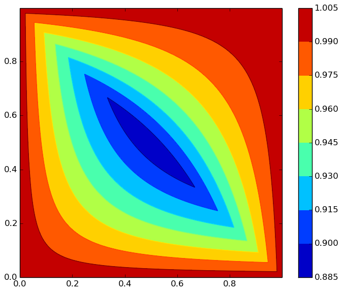Contour plot of the degree of approximation. It can be seen that the minimum degree of approximation occurs at the center point.

Plotting code:

import numpy as np
import matplotlib.pyplot as plt

x = np.arange(0, 1, 0.001)
y = np.arange(0, 1, 0.001)

X, Y = np.meshgrid(x, y)
Z1 = (1 + X + Y) / (1 + X + Y + X * Y)
Z2 = 2 * (X + Y) / (1 + X + Y + X * Y)
Z = (X + Y < 1) * Z1 + (X + Y >= 1) * Z2
plt.figure(figsize=(7, 6))
contourf = plt.contourf(X, Y, Z)
plt.contour(X, Y, Z)
plt.colorbar(contourf)
plt.show()

In essence, this error fundamentally depends on how well $\log_2 (1 + x)\approx x$ is approximated. We know that $x$ is the first-order Taylor expansion of the natural logarithm $\ln (1 + x)$, and $e=2.71828\dots$ is actually closer to 3, so if computers used base 3 instead, this algorithm would achieve higher average precision. In fact, there is indeed some theoretical analysis suggesting that the ideal base for computers is actually $e$, and 3 is closer to $e$ than 2 is, which is why ternary computers would be superior to binary ones in several respects. Both China and the former Soviet Union have researched ternary computers, but since binary is much easier to implement in hardware, binary computers still dominate today.

Bringing It into Deep Learning

That covers the introduction to the Mitchell approximation. Readers might be puzzled — isn't this the kind of thing that belongs to computer fundamentals and data structures? Why bother studying it? Does it even have any application in deep learning?

There are two reasons I studied it: first, it's genuinely beautiful and worth learning in its own right; second, it really can be applied in deep learning. In fact, I discovered it through a NeurIPS 2020 paper, Deep Neural Network Training without Multiplications, which validated on "ImageNet + ResNet50" that directly replacing the multiplications in a neural network with the additive form of the Mitchell approximation results in only a slight drop in accuracy — and possibly no drop at all.

Of course, the authors' current implementation only demonstrates that this substitution is acceptable in terms of effectiveness; in terms of speed, it's actually slower. This is because, although in theory replacing multiplication with approximate addition should always yield a speedup, realizing that speedup in practice requires optimization at the hardware level, since standard multiplication today has certainly already been optimized at the hardware level too. So the authors are really pointing toward a possible future direction for deep learning hardware optimization. Moreover, this isn't the first time the application of the Mitchell approximation in deep learning has been discussed — a quick Google search turns up two papers: Efficient Mitchell's Approximate Log Multipliers for Convolutional Neural Networks and Low-power implementation of Mitchell's approximate logarithmic multiplication for convolutional neural networks.

Readers might be reminded of Huawei's previously proposed additive neural network, AdderNet, whose goal is indeed similar in spirit, but which differs substantially in approach. AdderNet replaces the inner product in a neural network with the $l_1$ distance, thereby eliminating multiplication altogether; the paper discussed here, on the other hand, modifies how multiplication itself is implemented, reducing its computational cost, while potentially leaving existing neural network operations otherwise intact.

Old Wine, New Bottle

This post introduced the Mitchell approximation algorithm, published back in 1962 — an approximate method for computing logarithms and exponentials, on the basis of which we can convert multiplication into addition while retaining a reasonable degree of precision. It might look outdated on the surface, but repackage this algorithm in a "new bottle," and it becomes a NeurIPS 2020 paper.

So, what other bits of "old wine" have you found that could use a new bottle?