On the Vanishing/Exploding Gradient Problem of RNNs, Once More

也来谈谈RNN的梯度消失/爆炸问题 苏剑林 · 2020-11-13 · Machine Learning model optimization deep learning gradient

Although Transformer-based models have taken over most of the NLP landscape, RNN models such as LSTM and GRU still have their unique value in certain scenarios, so RNNs remain models well worth studying carefully. As for the analysis of RNN gradients, it's an excellent example of thinking about and analyzing models from an optimization perspective, and it deserves careful thought and understanding. After all, questions like "Why can LSTM solve the vanishing/exploding gradient problem?" are still among the popular interview questions today...

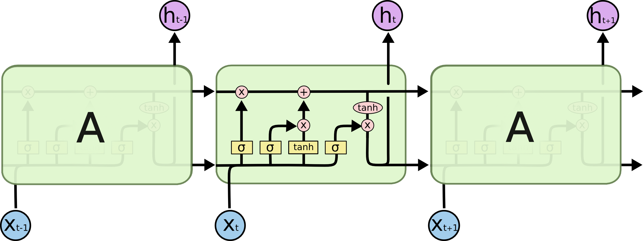Classic LSTM

Regarding this kind of question, quite a few people online have already offered answers. However, having looked through some articles (including some answers and columns on Zhihu, as well as classic English-language blog posts), I found that I couldn't locate a particularly good answer: some derivations use notation that's outright chaotic, some discussions fail to highlight the key points, and overall things don't feel clear or self-consistent enough. So I've tried to give my own understanding here, for readers' reference.

RNNs and Their Gradients

The unified definition of an RNN is

\begin{equation}h_t = f\left(x_t, h_{t-1};\theta\right)\end{equation}

where $h_t$ is the output at each step, jointly determined by the current input $x_t$ and the previous output $h_{t-1}$, and $\theta$ are the trainable parameters. For the most basic analysis, we can assume that $h_t,x_t,\theta$ are all one-dimensional, which gives us the most intuitive understanding, and whose results still carry reference value for the higher-dimensional case. The reason we care about gradients is that our mainstream optimizers today are still gradient descent and its variants, so we need the model we define to have a reasonably well-behaved gradient. We can compute:

\begin{equation}\frac{d h_t}{d\theta} = \frac{\partial h_t}{\partial h_{t-1}}\frac{d h_{t-1}}{d\theta} + \frac{\partial h_t}{\partial \theta}\end{equation}

As we can see, the gradient of an RNN is itself an RNN: the gradient at the current step $\frac{d h_t}{d\theta}$ is a function of the gradient at the previous step $\frac{d h_{t-1}}{d\theta}$ and the gradient of the current operation $\frac{\partial h_t}{\partial \theta}$. At the same time, from the formula above we can see that vanishing or exploding gradients are, in fact, almost inevitable: when $\left|\frac{\partial h_t}{\partial h_{t-1}}\right| < 1$, it means the historical gradient information decays, so after enough steps the gradient must vanish (much like $\lim\limits_{n\to\infty} 0.9^n \to 0$); when $\left|\frac{\partial h_t}{\partial h_{t-1}}\right| > 1$, since the historical gradient information keeps getting amplified, the gradient must explode after enough steps (much like $\lim\limits_{n\to\infty} 1.1^n \to \infty$). It's simply not possible for it to stay exactly at $\left|\frac{\partial h_t}{\partial h_{t-1}}\right| = 1$ forever. Of course, it's conceivable that at some time steps the value is greater than 1 and at others less than 1, ultimately hovering around 1, but the probability of that happening is very small — it would require a very carefully engineered model.

So as the number of steps grows, vanishing or exploding gradients are almost unavoidable; all we can do is mitigate the problem over a finite number of steps.

Vanishing or Exploding?

At this point we still haven't clarified one thing: what exactly do we mean by "vanishing/exploding gradients" in an RNN? Exploding gradients are easy to understand — the gradient values diverge, and eventually you get NaNs. But does "vanishing" mean the gradient becomes zero? Not quite. What we just described as gradient vanishing is that $\left|\frac{\partial h_t}{\partial h_{t-1}}\right|$ stays below 1, so the historical gradient keeps decaying — but that doesn't mean the total gradient becomes exactly 0. To be specific, if we keep iterating, we get

\begin{equation}\begin{aligned}\frac{d h_t}{d\theta} =& \frac{\partial h_t}{\partial h_{t-1}}\frac{d h_{t-1}}{d\theta} + \frac{\partial h_t}{\partial \theta}\\ =& \frac{\partial h_t}{\partial \theta}+\frac{\partial h_t}{\partial h_{t-1}}\frac{\partial h_{t-1}}{\partial \theta}+\frac{\partial h_t}{\partial h_{t-1}}\frac{\partial h_{t-1}}{\partial h_{t-2}}\frac{\partial h_{t-2}}{\partial \theta}+\dots\\ \end{aligned}\end{equation}

Clearly, as long as $\frac{\partial h_t}{\partial \theta}$ is nonzero, the probability that the total gradient is exactly 0 is actually quite small. But if we keep iterating indefinitely, the coefficient in front of the $\frac{\partial h_1}{\partial \theta}$ term is a product of $t-1$ terms, $\frac{\partial h_t}{\partial h_{t-1}}\frac{\partial h_{t-1}}{\partial h_{t-2}}\cdots\frac{\partial h_2}{\partial h_1}$; if all their absolute values are less than 1, then the result will tend to 0. In that case, $\frac{d h_t}{d\theta}$ ends up containing almost no information from the initial gradient $\frac{\partial h_1}{\partial \theta}$ at all — and this is exactly what "gradient vanishing" means in RNNs: the further back in time a step is, the less significant its feedback gradient signal becomes, until eventually it may have essentially no effect at all. This means the RNN's ability to capture long-range dependencies has effectively failed.

Put plainly: if your optimization process has essentially no connection to long-range feedback, how could you expect the learned model to effectively capture long-range dependencies?

A Few Mathematical Identities

Everything above was a general-purpose analysis; now let's turn to specific RNN variants. But before we do, we need to recall a few mathematical identities that we'll use repeatedly in the derivations below:

$$\begin{equation}\begin{aligned} &\tanh x = 2\sigma(2x) - 1\\ &\sigma(x) = \frac{1}{2}\left(\tanh \frac{x}{2} + 1\right)\\ &(\tanh x)' = 1 - \tanh^2 x\\ &\sigma'(x) = \sigma(x)\left(1 - \sigma(x)\right) \end{aligned}\end{equation}$$

where $\sigma(x) = 1/(1+e^{-x})$ is the sigmoid function. What these identities really say is this: $\tanh x$ and $\sigma(x)$ are essentially equivalent, and both of their derivatives can be expressed in terms of themselves.

Analysis of the Simple RNN

First up is the more primitive Simple RNN (sometimes we do literally call it "SimpleRNN"), whose formula is:

\begin{equation}h_t = \tanh \left(Wx_t + Uh_{t-1} + b\right)\end{equation}

where $W,U,b$ are the parameters to be optimized. At this point it's natural to raise a first question: why use $\tanh$ as the activation function rather than the more popular $\text{relu}$? Good question — we'll answer it shortly.

From the discussion above, we already know that whether the gradient vanishes or explodes mainly depends on $\left|\frac{\partial h_t}{\partial h_{t-1}}\right|$, so let's compute

\begin{equation}\frac{\partial h_t}{\partial h_{t-1}} = \left(1-h_t^2\right)U\label{eq:rnn-g}\end{equation}

Since we can't pin down the range of $U$, $\left|\frac{\partial h_t}{\partial h_{t-1}}\right|$ could be either less than or greater than 1, so there is indeed a risk of vanishing/exploding gradients. But here's the interesting part: if $|U|$ is large, then correspondingly $h_t$ will be very close to 1 or -1, which actually makes $\left(1-h_t^2\right)U$ small. In fact, one can rigorously prove that, for fixed $h_{t-1}\neq 0$, $\left(1-h_t^2\right)U$ as a function of $U$ is bounded — that is, no matter what value $U$ takes, it never exceeds some fixed constant.

This lets us answer why the activation function should be $\tanh$: because once we use $\tanh$ as the activation, the corresponding gradient $\frac{\partial h_t}{\partial h_{t-1}}$ is bounded. Although this bound need not be 1, a bounded quantity has a higher probability of staying under 1 than an unbounded one, so the risk of exploding gradients is lower. By contrast, if we used $\text{relu}$ activation, its derivative on the positive half-line is constantly 1, and in that case $\frac{\partial h_t}{\partial h_{t-1}}=U$ is unbounded, making the risk of exploding gradients higher.

So the main purpose of RNNs using $\text{tanh}$ rather than $\text{relu}$ is to mitigate the risk of exploding gradients. Of course, this mitigation is only relative — even with $\tanh$, explosion is still possible. In fact, the most fundamental way to handle exploding gradients is parameter clipping or gradient clipping: in other words, if we manually clip $U$ into $[-1,1]$, doesn't that guarantee the gradient won't explode? Naturally, some readers might then ask: if clipping solves the problem, can we just use $\text{relu}$? Indeed we can — with a good initialization scheme plus parameter/gradient clipping, an RNN using $\text{relu}$ can also be trained successfully. But we still prefer $\tanh$, precisely because its corresponding $\frac{\partial h_t}{\partial h_{t-1}}$ is bounded, so we don't need to clip as aggressively, and the model's fitting capacity may end up better as a result.

Results for LSTM

Of course, while clipping does work, it's ultimately a stopgap measure — and clipping can only address exploding gradients, not vanishing ones. If the problem can be solved through the model's design itself, that would naturally be preferable. The legendary LSTM is supposedly exactly such a design — but is that really the case? Let's analyze it right away.

The update equations of LSTM are more complex; they are:

\begin{equation}\begin{aligned} f_{t} & = \sigma \left( W_{f} x_{t} + U_{f} h_{t - 1} + b_{f} \right) \\ i_{t} & = \sigma \left( W_{i} x_{t} + U_{i} h_{t - 1} + b_{i} \right) \\ o_{t} & = \sigma \left( W_{o} x_{t} + U_{o} h_{t - 1} + b_{o} \right) \\ \hat{c}_t & = \tanh \left( W_{c} x_{t} + U_{c} h_{t - 1} + b_{c} \right)\\ c_{t} & = f_{t} \circ c_{t - 1} + i_{t} \circ \hat{c}_t \\ h_{t} & = o_{t} \circ \tanh \left( c_{t} \right)\end{aligned}\end{equation}

We could compute $\frac{\partial h_t}{\partial h_{t-1}}$ in the same way as before, but from $h_{t} = o_{t} \circ \tanh \left( c_{t} \right)$ we can see that analyzing $c_{t}$ is equivalent to analyzing $h_{t}$, and computing $\frac{\partial c_t}{\partial c_{t-1}}$ turns out to be simpler, so let's go in that direction.

Likewise, let's first focus on the 1-dimensional case. Using the derivative rules, we get

\begin{equation}\frac{\partial c_t}{\partial c_{t-1}}=f_t + c_{t-1}\frac{\partial f_t}{\partial c_{t-1}}+ \hat{c}_{t}\frac{\partial i_t}{\partial c_{t-1}}+ i_{t}\frac{\partial \hat{c}_t}{\partial c_{t-1}}\end{equation}

The first term on the right, $f_t$ — what we call the "forget gate" — turns out, as we'll show below, to be the "dominant term," since the other three terms are generally secondary. Since $f_t$ lies between 0 and 1, this means the risk of exploding gradients will be quite small. Whether gradients vanish depends on whether $f_t$ / $f_t$ stays close to 1. But quite conveniently, there's a remarkably self-consistent conclusion here: if our task heavily depends on historical information, then $f_t$ will tend to be close to 1, and in that case the historical gradient signal also happens to be resistant to vanishing; if $f_t$ is close to 0, that indicates our task doesn't depend on historical information, in which case it's fine even if the gradient does vanish.

So now the key question is whether the claim that "the other three terms are secondary" actually holds. The remaining three terms all take the form "one term times the partial derivative of another," and the terms being differentiated all involve $\sigma$ or $\tanh$ activations. As we noted earlier when recalling the mathematical identities, $\sigma$ and $\tanh$ are essentially equivalent, so the remaining three terms behave similarly — analyzing one of them is as good as analyzing the other two. Taking the second term as an example, substituting $h_{t-1} = o_{t-1} \tanh \left( c_{t-1} \right)$, we can compute

\begin{equation}c_{t-1}\frac{\partial f_t}{\partial c_{t-1}}=f_t \left(1 - f_t\right) o_{t-1} \left(1-\tanh^2 c_{t-1}\right)c_{t-1}U_f\end{equation}

Note that $f_t,1 - f_t,o_{t-1},$ all lie between 0 and 1, and one can also show that $\left|\left(1-\tanh^2 c_{t-1}\right)c_{t-1}\right| < 0.45$, so it too lies between -1 and 1. So $c_{t-1}\frac{\partial f_t}{\partial c_{t-1}}$ amounts to one factor of $U_f$ multiplied by four gates — the result gets squeezed to something much smaller. So as long as the initialization isn't disastrous, this term will be compressed to something quite small and won't dominate. Compared with the Simple RNN's gradient $\eqref{eq:rnn-g}$, it has three extra gates — so in plain terms, the change amounts to: "one gate alone can't crush you, but throw in a few more gates and see what happens."

The conclusions for the remaining two terms are similar:

\begin{equation}\begin{aligned} \hat{c}_{t}\frac{\partial i_t}{\partial c_{t-1}}=&\,i_t \left(1 - i_t\right) o_{t-1} \left(1-\tanh^2 c_{t-1}\right)\hat{c}_{t}U_i\\ i_{t}\frac{\partial \hat{c}_t}{\partial c_{t-1}}=&\,\left(1 - \hat{c}_t^2\right) o_{t-1} \left(1-\tanh^2 c_{t-1}\right)i_{t}U_c \end{aligned}\end{equation}

So, the latter three terms' gradients carry more "gates," and generally speaking, once multiplied together they get compressed even more heavily. As a result, the dominant term is still $f_t$: the fact that $f_t$ lies between 0 and 1 keeps the risk of exploding gradients low, while $f_t$ reflects the model's dependence on historical information, which happens to coincide with the degree to which historical gradients are preserved — these two facts are mutually consistent. So LSTM does a good job of alleviating the vanishing gradient problem as well. In summary, LSTM effectively mitigates both vanishing and exploding gradients simultaneously, which is why nowadays when training LSTMs, in most cases we simply need to call an adaptive-learning-rate optimizer like Adam — no manual gradient adjustment required.

Of course, these are all "general tendencies." If you deliberately try to construct an LSTM that suffers from vanishing/exploding gradients, you certainly can. Moreover, even though LSTM can mitigate these two problems, it can only do so within a limited number of steps — if your sequence is very long, say thousands or tens of thousands of steps, whatever is going to vanish will still vanish eventually. After all, relying on a single vector can't cache that much information.

A Quick Look at GRU

Before wrapping up, let's also give a quick analysis of LSTM's strong competitor, GRU. The computation of GRU proceeds as:

\begin{equation}\begin{aligned} z_{t} & = \sigma \left( W_{z} x_{t} + U_{z} h_{t - 1} + b_{z} \right) \\ r_{t} & = \sigma \left( W_{r} x_{t} + U_{r} h_{t - 1} + b_{r} \right) \\ \hat{h}_t & = \tanh \left( W_{h} x_{t} + U_{h} (r_t \circ h_{t - 1}) + b_{c} \right)\\ h_{t} & = \left(1 - z_{t}\right) \circ h_{t - 1} + z_{t} \circ \hat{h}_t \end{aligned}\end{equation}

There's an even more extreme variant that merges $r_t,z_t$ into one:

\begin{equation}\begin{aligned} r_{t} & = \sigma \left( W_{r} x_{t} + U_{r} h_{t - 1} + b_{r} \right) \\ \hat{h}_t & = \tanh \left( W_{h} x_{t} + U_{h} (r_t \circ h_{t - 1}) + b_{c} \right)\\ h_{t} & = \left(1 - r_{t}\right) \circ h_{t - 1} + r_{t} \circ \hat{h}_t \end{aligned}\end{equation}

Either way, we notice that when computing $\hat{h}_t$, $h_{t-1}$ is always first multiplied by a $r_t$ to become $r_t \circ h_{t - 1}$. I wonder if readers have ever found this puzzling? Wouldn't it be simpler and more intuitive to just use $h_{t-1}$ directly?

First, notice that $h_0$ is generally initialized to all zeros, and $\hat{h}_t$, because of the $\tanh$ activation, necessarily lies between -1 and 1. So $h_{t}$, being a weighted average of $h_{t-1}$ and $\hat{h}_t$, also always stays between -1 and 1 — meaning $h_t$ itself already behaves somewhat like a gate. This differs from LSTM's $c_t$, where in theory $c_t$ could potentially diverge. With this in mind, let's now take the derivative:

\begin{equation}\begin{aligned} \frac{\partial h_t}{\partial h_{t-1}} =& 1 - z_t - z_t (1-z_t) h_{t-1} U_z + z_t (1-z_t) \hat{h}_{t} U_z \\ & + \left(1-\hat{h}_{t}^2\right)r_t\left(1 + (1 - r_t)h_{t-1}U_r\right) z_t U_h \end{aligned}\end{equation}

The result is actually similar to LSTM's — the dominant term should still be $1-z_t$ — but the remaining terms have one fewer gate compared to their LSTM counterparts, so their magnitude could be larger, making them relatively more unstable than LSTM's gradients. In particular, the operation $r_t \circ h_{t - 1}$, while introducing one extra gate $r_t$ into the last term, simultaneously introduces an extra term $1 + (1 - r_t)h_{t - 1}U_r$ — whether that's good or bad is hard to say. Overall, my sense is that GRU is probably somewhat less stable than LSTM, and more dependent on good initialization.

Based on the above analysis, I personally think that if we want to keep the spirit of GRU's idea while simplifying LSTM and preserving LSTM's gradient-friendliness, a better design would be to move $r_t \circ h_{t - 1}$ to the end:

\begin{equation}\begin{aligned} z_{t} & = \sigma \left( W_{z} x_{t} + U_{z} h_{t - 1} + b_{z} \right) \\ r_{t} & = \sigma \left( W_{r} x_{t} + U_{r} h_{t - 1} + b_{r} \right) \\ \hat{c}_t & = \tanh \left( W_{h} x_{t} + U_{h} h_{t - 1} + b_{c} \right)\\ c_{t} & = \left(1 - z_{t}\right) \circ c_{t - 1} + z_{t} \circ \hat{c}_t \\ h_t & = r_t \circ c_t\end{aligned}\end{equation}

Of course, this requires caching an extra variable, which comes with additional GPU memory cost.

Summary

This article discussed the vanishing/exploding gradient problem in RNNs, examining, in a fairly clear-cut way, the gradient flow in RNN, LSTM, and GRU models through the lens of the boundedness of the gradient function and the number of gates involved, in order to gauge the relative risk of vanishing/exploding gradients in each. This piece was written somewhat in isolation, without much outside consultation, so if there are errors or omissions, I ask readers' forgiveness and welcome corrections.