Mitigating Class Imbalance via Mutual Information

通过互信息思想来缓解类别不平衡问题 苏剑林 · 2020-07-19 · Machine Learning optimization mutual information loss function

Class imbalance, also known as the "long-tail problem," is one of the most common challenges in machine learning, especially for datasets drawn from real-world scenarios, which are almost always class-imbalanced. About two years ago I was also thinking about this problem, and at the time I happened to have some insights into "mutual information," so I came up with a solution based on mutual-information ideas. But after mulling it over, the approach seemed a bit too trivial, so I didn't pursue it further. However, a few days ago I came across a Google paper on arXiv, Long-tail learning via logit adjustment, and was surprised to find that it contains a method almost identical to what I had originally conceived. That's when I realized the idea I had abandoned back then could actually achieve SOTA performance! So, drawing on this paper, I've organized my original train of thought here, and I hope readers won't mind the "hindsight-is-20/20" nature of this post.

Problem Description

Here we're mainly concerned with the single-label multi-class classification problem. Suppose there are $1,2,\cdots,K$ classes in total, numbering $K$, the training data is $(x,y)\sim\mathcal{D}$, and the distribution we model is $p_{\theta}(y|x)$. Then our optimization objective is maximum likelihood, or equivalently, minimizing the cross-entropy:

\begin{equation}\mathop{\text{argmin}}_{\theta}\,\mathbb{E}_{(x,y)\sim\mathcal{D}}[-\log p_{\theta}(y|x)]\end{equation}

Typically, the last step of the probability model we build is a softmax. Suppose the result before the softmax is $f(x;\theta)$ (i.e., the logits), then

\begin{equation}-\log p_{\theta}(y|x)=-\log \frac{e^{f_y(x;\theta)}}{\sum\limits_{i=1}^K e^{f_i(x;\theta)}}=\log\left[1 + \sum_{i\neq y}e^{f_i(x;\theta) - f_y(x;\theta)}\right]\label{eq:loss-1}\end{equation}

So-called class imbalance refers to the situation where a few classes have a huge number of samples, much like "20% of the people hold 80% of the wealth." The remaining classes are numerous, but each has very few samples, so if you sort them from most to least frequent, it looks like there's a long "tail" trailing off — hence the name "long-tail phenomenon." In such cases, when we sample a batch during training, we rarely get a chance to sample the low-frequency classes, so the model easily ends up neglecting them. But at evaluation time, we usually care more about how well the model recognizes those low-frequency classes — and that's precisely where the contradiction lies.

Common Approaches

Readers have probably already heard of the common approaches, which broadly fall into three directions:

1. Starting from the data: use oversampling or undersampling so that each batch becomes more balanced across classes;
2. Starting from the loss: a classic approach is to divide the loss of samples from class $y$ by the frequency $p(y)$ of that class;
3. Starting from the outputs: after training a model normally, make adjustments at the prediction stage to favor low-frequency classes — for example, if positive samples are far fewer than negative ones, we might treat any prediction above 0.2 (rather than 0.5) as positive.

Google's original paper cites quite a few references for each of these three directions; readers interested in a deeper survey can go read the original paper directly. There's also a Zhihu article, Long-Tailed Classification (2): Recent Research on Classification under Long-Tailed Distributions, which introduces this problem as well, and readers may want to check it out.

Learning Mutual Information

Let's think back to how we determine that a classification problem is imbalanced in the first place. Clearly, the usual approach is to tally up the frequency $p(y)$ of each class over the entire training set, and then find that $p(y)$ is concentrated in just a handful of classes. So the key to solving the class-imbalance problem is figuring out how to incorporate this prior knowledge, $p(y)$, into the model.

When I was previously working out a word embedding model (see the post A More Elegant Word Embedding Model (II): Modeling Language), I emphasized that, compared with fitting conditional probabilities, if a model can directly fit mutual information, it will learn something more fundamental, because mutual information is the quantity that truly reveals the core association. However, fitting mutual information directly is not so easy to train, whereas conditional probability is easy to train — you just use cross-entropy $-\log p_{\theta}(y|x)$ directly. So a fairly appealing idea is: can we get the model to still use cross-entropy as the loss, while essentially fitting mutual information underneath?

In equation $\eqref{eq:loss-1}$, we were modeling

\begin{equation}p_{\theta}(y|x)=\frac{e^{f_y(x;\theta)}}{\sum\limits_{i=1}^K e^{f_i(x;\theta)}}\end{equation}

Now let's switch to modeling mutual information instead, i.e., we want

\begin{equation}\log \frac{p_{\theta}(y|x)}{p(y)}\sim f_y(x;\theta)\quad \Leftrightarrow\quad \log p_{\theta}(y|x)\sim f_y(x;\theta) + \log p(y)\end{equation}

Re-normalizing with softmax according to the right-hand side form gives us $p_{\theta}(y|x)=\frac{e^{f_y(x;\theta)+\log p(y)}}{\sum\limits_{i=1}^K e^{f_i(x;\theta)+\log p(i)}}$, or written as a loss:

\begin{equation}-\log p_{\theta}(y|x)=-\log \frac{e^{f_y(x;\theta)+\log p(y)}}{\sum\limits_{i=1}^K e^{f_i(x;\theta)+\log p(i)}}=\log\left[1 + \sum_{i\neq y}\frac{p(i)}{p(y)}e^{f_i(x;\theta) - f_y(x;\theta)}\right]\label{eq:loss-2}\end{equation}

The original paper calls this the logit adjustment loss. More generally, we can also add a tuning factor $\tau$:

\begin{equation}-\log p_{\theta}(y|x)=-\log \frac{e^{f_y(x;\theta)+\tau\log p(y)}}{\sum\limits_{i=1}^K e^{f_i(x;\theta)+\tau\log p(i)}}=\log\left[1 + \sum_{i\neq y}\left(\frac{p(i)}{p(y)}\right)^{\tau}e^{f_i(x;\theta) - f_y(x;\theta)}\right]\label{eq:loss-3}\end{equation}

In most cases, $\tau=1$ already gives near-optimal results. If the last layer of $f_y(x;\theta)$ has a bias term, then the simplest way to implement this is to initialize that bias term as $\tau\log p(y)$. It can also be written directly into the loss function:

import numpy as np
import keras.backend as K

def categorical_crossentropy_with_prior(y_true, y_pred, tau=1.0):
    """带先验分布的交叉熵
    注：y_pred不用加softmax
    """
    prior = xxxxxx  # 自己定义好prior，shape为[num_classes]
    log_prior = K.constant(np.log(prior + 1e-8))
    for _ in range(K.ndim(y_pred) - 1):
        log_prior = K.expand_dims(log_prior, 0)
    y_pred = y_pred + tau * log_prior
    return K.categorical_crossentropy(y_true, y_pred, from_logits=True)

def sparse_categorical_crossentropy_with_prior(y_true, y_pred, tau=1.0):
    """带先验分布的稀疏交叉熵
    注：y_pred不用加softmax
    """
    prior = xxxxxx  # 自己定义好prior，shape为[num_classes]
    log_prior = K.constant(np.log(prior + 1e-8))
    for _ in range(K.ndim(y_pred) - 1):
        log_prior = K.expand_dims(log_prior, 0)
    y_pred = y_pred + tau * log_prior
    return K.sparse_categorical_crossentropy(y_true, y_pred, from_logits=True)

Analysis of the Results

Clearly, the logit adjustment loss is also one of the loss-adjustment schemes; the difference is that it adjusts the weighting inside $\log$, whereas the conventional approach adjusts things outside $\log$. As for its benefits, they're exactly the benefits of mutual information: mutual information reveals the associations that truly matter, so adding a prior-distribution bias to the logits lets the model "solve with the prior whatever can be solved with the prior, and let the model handle only the essential part that the prior cannot."

At the prediction stage, depending on the evaluation metric, we can devise different prediction schemes. From Notes on Function Smoothing: Differentiable Approximations to Non-differentiable Functions we know that, for overall accuracy, we have the approximation

\begin{equation}\text{overall accuracy} \approx \frac{1}{N}\sum_{i=1}^N p_{\theta}(y_i|x_i)\end{equation}

where $\{(x_i,y_i)\}_{i=1}^N$ is the validation set. So if we're not worried about class imbalance and are simply pursuing higher overall accuracy, then for each $x$ we should directly output the class with the largest $p_{\theta}(y|x)$. But if we want the accuracy on each class to be as high as possible, we can rewrite the above expression as

\begin{equation}\text{overall accuracy} \approx \frac{1}{N}\sum_{i=1}^N \frac{p_{\theta}(y_i|x_i)}{p(y_i)}\times p(y_i)=\sum_{y=1}^K p(y)\left(\frac{1}{N}\sum_{x_i\in\Omega_y} \frac{p_{\theta}(y|x_i)}{p(y)}\right)\end{equation}

where $\Omega_y=\{x_i|y_i=y,i=1,2,\cdots,N\}$ is also the set of $x$ with label $y$; the right-hand side of the equality is really just grouping together the terms belonging to the same $y$. We know that "overall accuracy = weighted average of per-class accuracies," and the expression above happens to have exactly that form, so the term $\frac{1}{N}\sum\limits_{x_i\in\Omega_y} \frac{p_{\theta}(y|x_i)}{p(y)}$ inside the parentheses is an approximation of the "per-class accuracy." Therefore, if we want the accuracy on every class to be as high as possible, we should output whichever class maximizes $\frac{p_{\theta}(y|x)}{p(y)}$ (without weighting). Combining this with the form of $p_{\theta}(y|x)$, we arrive at the conclusion

\begin{equation}y^{*}=\left\{\begin{aligned}&\mathop{\text{argmax}}\limits_y\, f_y(x;\theta)+\tau\log p(y),\quad(\text{pursue overall accuracy})\\ &\mathop{\text{argmax}}\limits_y\, f_y(x;\theta),\quad(\text{want per-class accuracy uniform}) \end{aligned}\right.\end{equation}

The first case is simply outputting the class with the largest conditional probability, while the second is outputting the class with the largest mutual information — you choose whichever suits your specific needs.

As for the detailed experimental results, you can go read the paper yourself; suffice it to say they're good enough to be a little surprising:

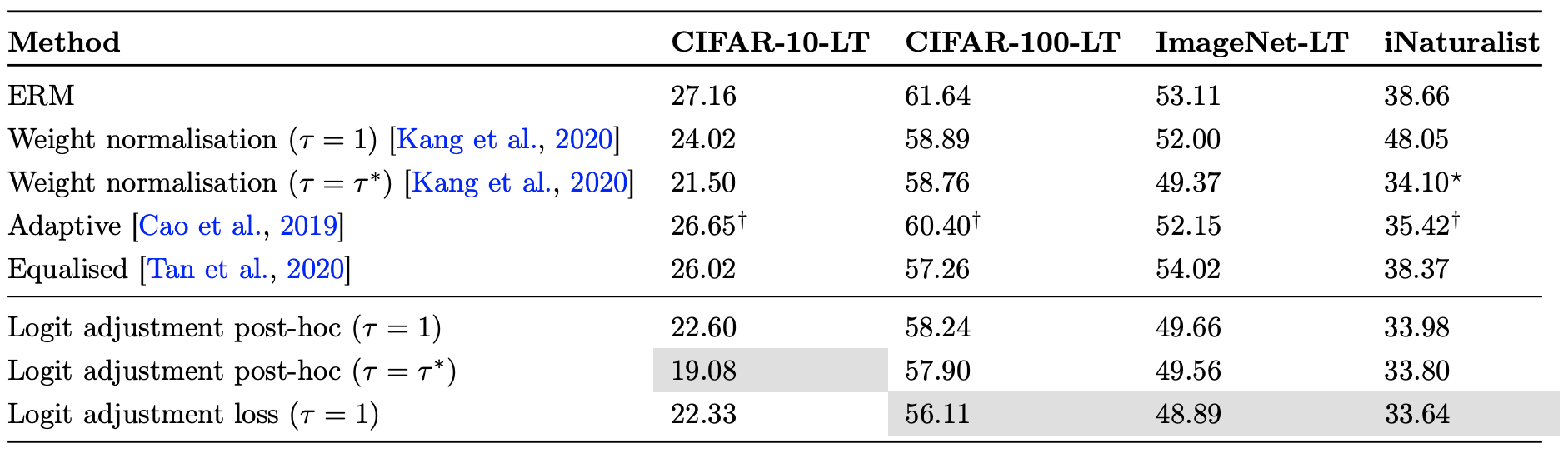Experimental results from the original paper

Summary

This post gave a brief introduction to a mutual-information-based approach for handling class imbalance. I had once conceived of this scheme myself but never pursued it further, and a recent Google paper turned out to present the same method — so I've recorded and analyzed it briefly here. In the end, Google's experimental results show that this method can achieve SOTA-level performance.