JoSE: Word and Sentence Embeddings on the Sphere

JoSE：球面上的词向量和句向量 苏剑林 · 2019-11-11 · Machine Learning geometry NLP word vector NLP

This article introduces a word/sentence embedding model called JoSE (Joint Spherical Embedding), published at NeurIPS 2019, from the paper Spherical Text Embedding. JoSE inherits its ideas and methodology from Doc2Vec, and its evaluation results are quite impressive, but the writing feels somewhat overblown. Still, I decided to write this piece because I find some of the analysis in the paper genuinely interesting, and it may offer useful reference value for optimization problems in general.

Optimization Objective

Conceptually, this paper is essentially aligned with Doc2Vec: to train sentence vectors, each sentence is represented by an id, treated as if it were itself a word that co-occurs with every word in the sentence, and then a Skip-Gram model is trained via negative sampling. Where JoSE differs from Doc2Vec is that it normalizes the norm of every vector (i.e., it only considers vectors on the unit sphere), and instead of cross-entropy, it uses a hinge loss as the training objective:

\begin{equation}\max(0, m - \cos(\boldsymbol{u}, \boldsymbol{v}) - \cos(\boldsymbol{u}, \boldsymbol{d}) + \cos(\boldsymbol{u}', \boldsymbol{v}) + \cos(\boldsymbol{u}', \boldsymbol{d})\label{eq:loss}\end{equation}more

Here $\boldsymbol{u}$ is the word vector of the "center word," $\boldsymbol{v}$ is the word vector of the "context word" — the two come from separate embedding spaces — $\boldsymbol{d}$ is the sentence vector of the current sentence, $\boldsymbol{u}'$ is the "center word" vector obtained via negative sampling, and $m > 0$ is a constant. Readers who have worked with similarity models before should be able to easily read off what this objective means: it wants the "word-word-sentence" score $\cos(\boldsymbol{u}, \boldsymbol{v}) + \cos(\boldsymbol{u},\boldsymbol{d})$ within the sentence to exceed the "word-random word-sentence" score $\cos(\boldsymbol{u}', \boldsymbol{v}) + \cos(\boldsymbol{u}', \boldsymbol{d})$, but it need not be too much higher—exceeding it by $m$ is enough.

Assuming $\boldsymbol{u},\boldsymbol{v},\boldsymbol{d}$ are all already normalized, the objective $\eqref{eq:loss}$ becomes (with each vector treated as a column vector):

\begin{equation}\max(0, m - \boldsymbol{v}^{\top}\boldsymbol{u} - \boldsymbol{d}^{\top}\boldsymbol{u} + \boldsymbol{v}^{\top} \boldsymbol{u}' + \boldsymbol{d}^{\top} \boldsymbol{u}')\label{eq:loss2}\end{equation}

Gradient Descent

There's nothing particularly novel about the objective $\eqref{eq:loss}$ or $\eqref{eq:loss2}$ — like most word-embedding objectives, it measures word relatedness using an inner product, except here the vectors are normalized, so the inner product is just $\cos$. As for whether hinge loss or cross-entropy is better, I don't think it makes much of a difference.

What I actually find interesting is the paper's subsequent geometric analysis of the gradient. Let me reproduce the derivation here in my own words. Let $\boldsymbol{x}$ be one of the vectors among all the $\boldsymbol{u},\boldsymbol{v},\boldsymbol{d}$ vectors, and suppose we now fix all the other vectors and only optimize $\boldsymbol{x}$. Let the total loss be $f(\boldsymbol{x})$; this optimization problem can then be described in two equivalent ways:

\begin{equation}\mathop{\text{argmin}}_{\boldsymbol{x},\,\Vert\boldsymbol{x}\Vert=1} f(\boldsymbol{x})\quad\text{or}\quad \mathop{\text{argmin}}_{\boldsymbol{\theta}} f\left(\frac{\boldsymbol{\theta}}{\Vert \boldsymbol{\theta}\Vert}\right) \end{equation}

That is, we can think of this as minimizing $f(\boldsymbol{x})$ subject to the constraint $\Vert \boldsymbol{x}\Vert=1$, or alternatively, by setting $\boldsymbol{x}=\boldsymbol{\theta}/\Vert\boldsymbol{\theta}\Vert$, we can convert it into an unconstrained minimization of $f(\boldsymbol{\theta}/\Vert\boldsymbol{\theta}\Vert)$. Since we're less familiar with constrained optimization, let's go with the latter interpretation.

Unlike more complex models, word embeddings are a relatively simple model, so it's best to derive the gradient by hand and write the corresponding function to perform gradient descent, rather than relying on automatic differentiation tools. For $f(\boldsymbol{\theta}/\Vert\boldsymbol{\theta}\Vert)$, it's not hard to derive that

\begin{equation}\nabla_{\boldsymbol{\theta}}\,f\left(\frac{\boldsymbol{\theta}}{\Vert \boldsymbol{\theta}\Vert}\right) = \frac{1}{\Vert\boldsymbol{\theta}\Vert}\left(\boldsymbol{I} - \boldsymbol{x}\boldsymbol{x}^{\top}\right)\nabla_{\boldsymbol{x}}\,f\left(\boldsymbol{x}\right) \end{equation}

where some variables have already been replaced by $\boldsymbol{x}=\boldsymbol{\theta}/\Vert\boldsymbol{\theta}\Vert$. Based on this result, the gradient descent update rule is

\begin{equation}\boldsymbol{\theta}_{t+1} = \boldsymbol{\theta}_{t} - \eta_t\left(\boldsymbol{I} - \boldsymbol{x}_t\boldsymbol{x}_t^{\top}\right)\nabla_{\boldsymbol{x}_t}\,f\left(\boldsymbol{x}_t\right) \end{equation}

where $\eta_t$ is the learning rate at the current step, and since the factor $1/\Vert\boldsymbol{\theta}\Vert$ is just a scalar, it has been folded into the learning rate. We can similarly write:

\begin{equation}\begin{aligned}\boldsymbol{x}_{t+1} = \frac{\boldsymbol{\theta}_{t+1}}{\Vert \boldsymbol{\theta}_{t+1}\Vert} =& \frac{\boldsymbol{\theta}_{t} - \eta_t\left(\boldsymbol{I} - \boldsymbol{x}_t\boldsymbol{x}_t^{\top}\right)\nabla_{\boldsymbol{x}_t}\,f\left(\boldsymbol{x}_t\right)}{\left\Vert \boldsymbol{\theta}_{t} - \eta_t\left(\boldsymbol{I} - \boldsymbol{x}_t\boldsymbol{x}_t^{\top}\right)\nabla_{\boldsymbol{x}_t}\,f\left(\boldsymbol{x}_t\right)\right\Vert}\\ =& \frac{\boldsymbol{x}_{t} - \eta_t/\Vert\boldsymbol{\theta}\Vert\times\left(\boldsymbol{I} - \boldsymbol{x}_t\boldsymbol{x}_t^{\top}\right)\nabla_{\boldsymbol{x}_t}\,f\left(\boldsymbol{x}_t\right)}{\left\Vert \boldsymbol{x}_{t} - \eta_t/\Vert\boldsymbol{\theta}\Vert\times\left(\boldsymbol{I} - \boldsymbol{x}_t\boldsymbol{x}_t^{\top}\right)\nabla_{\boldsymbol{x}_t}\,f\left(\boldsymbol{x}_t\right)\right\Vert} \end{aligned}\end{equation}

Again folding $1/\Vert\boldsymbol{\theta}\Vert$ into the learning rate, we obtain an update formula involving only $\boldsymbol{x}_t$:

\begin{equation}\boldsymbol{x}_{t+1} = \frac{\boldsymbol{x}_{t} - \eta_t\left(\boldsymbol{I} - \boldsymbol{x}_t\boldsymbol{x}_t^{\top}\right)\nabla_{\boldsymbol{x}_t}\,f\left(\boldsymbol{x}_t\right)}{\left\Vert \boldsymbol{x}_{t} - \eta_t\left(\boldsymbol{I} - \boldsymbol{x}_t\boldsymbol{x}_t^{\top}\right)\nabla_{\boldsymbol{x}_t}\,f\left(\boldsymbol{x}_t\right)\right\Vert}\end{equation}

Correcting the Update

So far, everything above has been a fairly standard derivation. Now comes the part I find genuinely interesting. First, we have

\begin{equation}\begin{aligned}\boldsymbol{g}=&\left(\boldsymbol{I} - \boldsymbol{x}_t\boldsymbol{x}_t^{\top}\right)\nabla_{\boldsymbol{x}_t}\,f\left(\boldsymbol{x}_t\right)\\ =&\nabla_{\boldsymbol{x}_t}\,f\left(\boldsymbol{x}_t\right) - \boldsymbol{x}_t\boldsymbol{x}_t^{\top}\nabla_{\boldsymbol{x}_t}\,f\left(\boldsymbol{x}_t\right)\\ =&\nabla_{\boldsymbol{x}_t}\,f\left(\boldsymbol{x}_t\right) - \boldsymbol{x}_t\Vert \nabla_{\boldsymbol{x}_t}\,f\left(\boldsymbol{x}_t\right)\Vert \cos\left(\boldsymbol{x}_t,\nabla_{\boldsymbol{x}_t}\,f\left(\boldsymbol{x}_t\right)\right) \end{aligned} \end{equation}

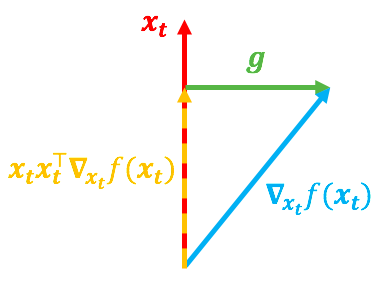
We can see that $\boldsymbol{x}_t\boldsymbol{x}_t^{\top}\nabla_{\boldsymbol{x}_t}\,f\left(\boldsymbol{x}_t\right)$ is precisely the projection component of the vector $\nabla_{\boldsymbol{x}_t}\,f\left(\boldsymbol{x}_t\right)$ along the direction of $\boldsymbol{x}_t$, and the whole of $\boldsymbol{g}$ is a vector perpendicular to $\boldsymbol{x}_t$, as illustrated below:

Geometric illustration of the gradient

In the figure above, the red vector represents $\boldsymbol{x}_t$ and the blue vector represents $\nabla_{\boldsymbol{x}_t}\,f\left(\boldsymbol{x}_t\right)$. Without the constraint $\Vert \boldsymbol{x}\Vert=1$, the update would be determined directly by $\nabla_{\boldsymbol{x}_t}\,f\left(\boldsymbol{x}_t\right)$, but because of the constraint, the update is instead determined by $\boldsymbol{g}=\left(\boldsymbol{I} - \boldsymbol{x}_t\boldsymbol{x}_t^{\top}\right)\nabla_{\boldsymbol{x}_t}\,f\left(\boldsymbol{x}_t\right)$. However, two different situations for $\nabla_{\boldsymbol{x}_t}\,f\left(\boldsymbol{x}_t\right)$ can both lead to the same $\boldsymbol{g}$:

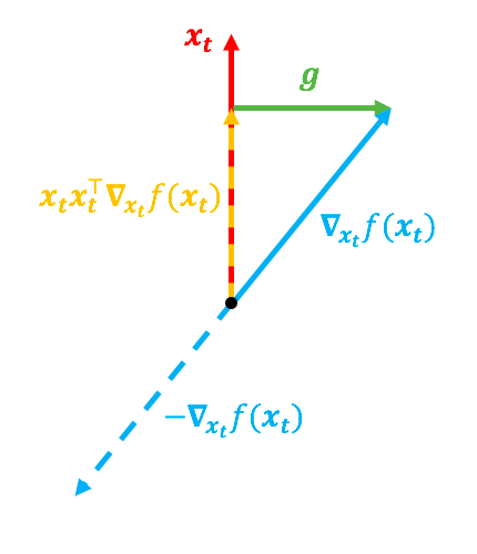First case: ∇xf(x) points in nearly the same direction as x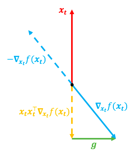Second case: ∇xf(x) points in nearly the opposite direction to x

In the first case, the direction of $\nabla_{\boldsymbol{x}_t}\,f\left(\boldsymbol{x}_t\right)$ is very close to that of $\boldsymbol{x}_t$; in the second case, it's the opposite. Yet in both cases, $\boldsymbol{g}$ is the same. As mentioned earlier, without the constraint, $\nabla_{\boldsymbol{x}_t}\,f\left(\boldsymbol{x}_t\right)$ would be the gradient, meaning $-\nabla_{\boldsymbol{x}_t}\,f\left(\boldsymbol{x}_t\right)$ would be a sensible update direction. Now that we have the constraint, $-\nabla_{\boldsymbol{x}_t}\,f\left(\boldsymbol{x}_t\right)$ can no longer indicate the most sensible gradient direction, but intuitively it should still be related to the update.

In the first case, $-\nabla_{\boldsymbol{x}_t}\,f\left(\boldsymbol{x}_t\right)$ and $\boldsymbol{x}_t$ point in fairly different directions, which suggests the update should be relatively large in this case; in the second case, $-\nabla_{\boldsymbol{x}_t}\,f\left(\boldsymbol{x}_t\right)$ and $\boldsymbol{x}_t$ point in nearly the same direction, and since we only care about the direction of $\boldsymbol{x}_{t+1}$, not its magnitude, the update in this case should presumably be smaller.

So even though $\boldsymbol{g}$ is the same in both cases, we still need to distinguish between them. A very natural idea is: since the degree of alignment between $-\nabla_{\boldsymbol{x}_t}\,f\left(\boldsymbol{x}_t\right)$ and $\boldsymbol{x}_t$ affects the size of the update, we might as well use

\begin{equation}1-\cos(-\nabla_{\boldsymbol{x}_t}\,f\left(\boldsymbol{x}_t\right),\boldsymbol{x}_t)=1+\frac{\boldsymbol{x}_t^{\top}\nabla_{\boldsymbol{x}_t}\,f\left(\boldsymbol{x}_t\right)}{\left\Vert \nabla_{\boldsymbol{x}_t}\,f\left(\boldsymbol{x}_t\right)\right\Vert} \end{equation}

to modulate the magnitude of the update. This modulation factor precisely has the property that "the more aligned the directions, the smaller the factor." This natural idea leads to the final update formula:

\begin{equation}\boldsymbol{x}_{t+1} = \frac{\boldsymbol{x}_{t} - \eta_t\left(1+\frac{\boldsymbol{x}_t^{\top}\nabla_{\boldsymbol{x}_t}\,f\left(\boldsymbol{x}_t\right)}{\left\Vert \nabla_{\boldsymbol{x}_t}\,f\left(\boldsymbol{x}_t\right)\right\Vert}\right)\left(\boldsymbol{I} - \boldsymbol{x}_t\boldsymbol{x}_t^{\top}\right)\nabla_{\boldsymbol{x}_t}\,f\left(\boldsymbol{x}_t\right)}{\left\Vert \boldsymbol{x}_{t} - \eta_t\left(1+\frac{\boldsymbol{x}_t^{\top}\nabla_{\boldsymbol{x}_t}\,f\left(\boldsymbol{x}_t\right)}{\left\Vert \nabla_{\boldsymbol{x}_t}\,f\left(\boldsymbol{x}_t\right)\right\Vert}\right)\left(\boldsymbol{I} - \boldsymbol{x}_t\boldsymbol{x}_t^{\top}\right)\nabla_{\boldsymbol{x}_t}\,f\left(\boldsymbol{x}_t\right)\right\Vert}\end{equation}

Overblown Presentation

Having covered the interesting parts, let's now talk about the parts I find less compelling. Any reader with a bit of background in NLP — who has seen the mathematics of Word2Vec and has derived the gradients of standard models — should feel that the first two sections above contain nothing particularly deep. The geometric interpretation and learning-rate adjustment in the third section are somewhat novel, but they're also traceable and reasonably straightforward. However, if you read the original paper, the impression you get is completely different: the author uses language like "probability distributions" and "optimization on Riemannian manifolds" to describe content that should be fairly easy to understand, but ends up making it thoroughly confusing — it really does feel like showing off for the sake of it.

First, what I find most puzzling is that the author starts off with an unreasonable assumption (making the word vectors continuous), and then spends considerable space arguing that $p(v|u)\sim e^{\cos(\boldsymbol{v},\boldsymbol{u})}$ and $p(u|d)\sim e^{\cos(\boldsymbol{u},\boldsymbol{d})}$ correspond to a Von Mises–Fisher distribution. And then? Nothing. Everything that follows has essentially nothing to do with this Von Mises–Fisher distribution, so I don't understand what purpose this section serves.

Then, in the optimization section, the author claims that minimizing $f(\boldsymbol{x})$ under the constraint $\Vert\boldsymbol{x}\Vert=1$ can't be done with ordinary gradient descent, so "Riemannian gradient descent" must be used instead — and then the showmanship begins: first Riemannian manifolds, then the general exponential map, then the Riemannian gradient. After all this elaborate machinery, what's left in the end is just a scheme that everyone can understand: $\boldsymbol{x}=\boldsymbol{\theta}/\Vert\boldsymbol{\theta}\Vert$. At this point I have to admit I'm impressed — though the author's logic and derivation are flawless, after all that maneuvering, the audience is left with the plain, simple result $\boldsymbol{x}=\boldsymbol{\theta}/\Vert\boldsymbol{\theta}\Vert$. So why not just discuss the optimization of $f(\boldsymbol{x}=\boldsymbol{\theta}/\Vert\boldsymbol{\theta}\Vert)$ directly from the start? Why drag ordinary readers through a Riemannian manifold detour just to confuse them?

Moreover, even the part I said I found genuinely interesting — the geometric interpretation of the update and the resulting modulation factor — is presented by the author in a rather muddled way. All in all, I think the theoretical derivation in this paper is loaded in many places with unnecessary jargon that needlessly increases the difficulty for ordinary readers.

Let me stress, finally, that I have never been against "multiple solutions to one problem," nor against elaborating and abstracting simple content, because such elaboration and abstraction can indeed yield a more comprehensive understanding, or reveal connections between different branches. But this kind of elaboration and abstraction should be built on top of a simple solution that most people can understand — not achieved by deliberately discarding the simple, understandable solution for the sake of elaboration and abstraction.

Experimental Results

Complaints aside, JoSE performs quite well in the experimental section. First, the authors provide an efficient C implementation of JoSE:

GitHub: https://github.com/yumeng5/Spherical-Text-Embedding

I tried it out myself, and training is indeed very fast; the resulting word/sentence vectors can be loaded using gensim's KeyedVectors. I also looked through the source code, which is concise and clear, and easy to modify for further experimentation.

As for the experimental results, JoSE is also quite strong on the word/sentence embedding evaluations presented in the paper:

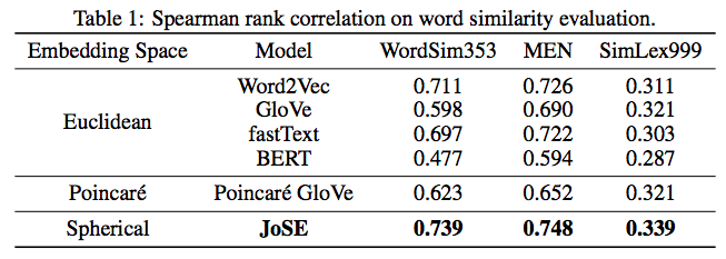Word similarity evaluation

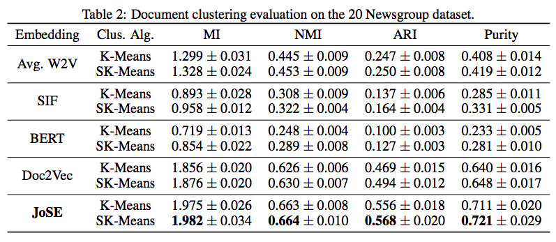Text clustering evaluation

Summary

This article introduced JoSE, a text embedding model published at NeurIPS 2019, focusing on the parts I found most inspiring and presenting the derivation in my own way. JoSE can be seen as a natural variant of Doc2Vec, refined in subtle ways, with the authors offering their own insights into the optimization method. Setting aside some seemingly overblown presentation choices, it remains a solid and noteworthy piece of work.