The Minimum Entropy Principle (V): "Layer by Layer" — Community Detection and Clustering

最小熵原理（五）：“层层递进”之社区发现与聚类 苏剑林 · 2019-10-19 · Machine Learning entropy clustering unsupervised minimum entropy

Let's tirelessly review the basics once more: the minimum entropy principle is an unsupervised-learning principle, in which "entropy" represents the cost of learning, and reducing this learning cost is our relentless pursuit. By "minimizing the learning cost," we can learn many results that align with our intuition in an unsupervised manner — this is the basic idea behind the minimum entropy principle.

In this article, we'll introduce a rather elegant clustering algorithm that likewise embodies the minimum entropy principle — indeed, it can be derived from it. It is called InfoMap, also known as MapEquation. In fact, InfoMap dates all the way back to 2007; the earliest paper is Maps of random walks on complex networks reveal community structure. Although it looks old, I still consider it the most elegant clustering algorithm around today, because it not only tells us "how to cluster," but more importantly gives us an elegant information-theoretic explanation of "why we should cluster," and derives the entire clustering procedure directly from that explanation.

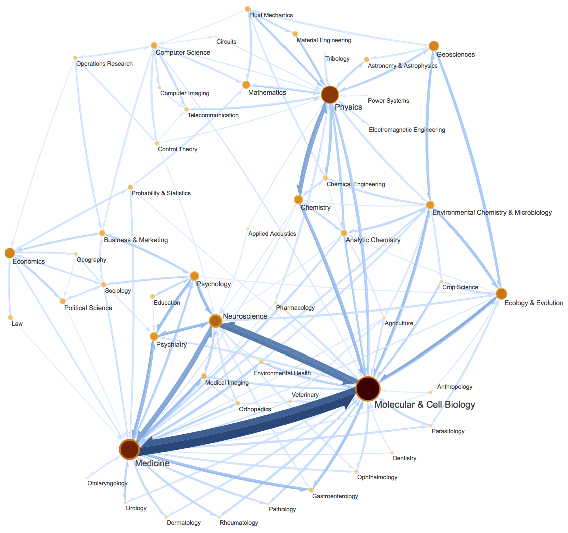A schematic diagram of a complex directed graph network. Image taken from the original InfoMap paper "Maps of random walks on complex networks reveal community structure"

Of course, its scope is not limited to clustering alone. More precisely, it is a "community detection" algorithm on graph networks. Community detection roughly means: given a directed/undirected graph network, find the "clumping" structure within that network. For the detailed meaning, readers can search for it themselves. In short, it's similar to clustering but carries richer meaning. (See also What is Community Detection?) more

Entropy and Coding

In previous articles, we've consistently used the concept of information entropy to describe related notions. Starting from this article, we'll introduce an equivalent concept — average code length — which will help us understand and construct the minimum-entropy objective more precisely.

Binary Tree Coding

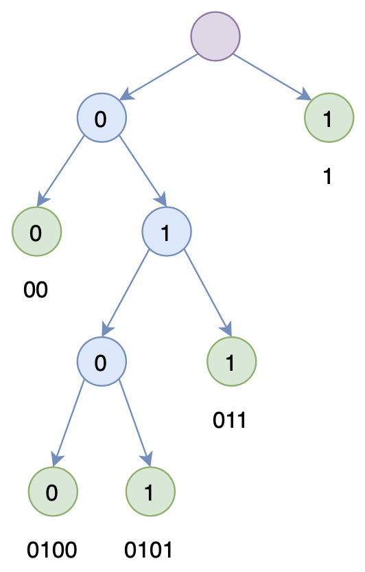No code is a prefix of any other code, so these codes can be organized into a binary tree

Coding, in essence, means representing raw information using combinations of a finite set of symbols, the most typical case being binary coding, which uses only the two digits 0 and 1. Codes and original objects are usually in one-to-one correspondence; for instance, "科" ("science") might correspond to 11, and "学" ("study") to 1001, so "科学" ("science") would correspond to (11, 1001).

Note that here we're considering static coding, meaning each encoded object corresponds one-to-one with a code, and we are considering coding without delimiters, meaning we don't need extra separators to decode individual objects. This only requires that no code be a prefix of any other code (so that we can keep reading the code stream until we identify one encoded object, then start reading again for the next). This means all the codes can be organized into a binary tree, where each code corresponds to a leaf of this tree, as shown in the figure.

Building on this, we can obtain a rather interesting and meaningful conclusion: suppose there are $n$ distinct symbols with code lengths $l_1,l_2,\cdots,l_n$ respectively, then we have

\begin{equation}\sum_{i=1}^n 2^{-l_i}\leq 1\label{eq:leq}\end{equation}

This is in fact a direct consequence of the binary-tree representation, and readers are encouraged to try proving it themselves.

Shortest Code Length

Now imagine a "speed stenography" scenario, where we need to quickly jot down the text we hear, recording each character with a binary code (let's set aside for now the question of how a person remembers the mapping between characters and codes). To write faster, we obviously want frequently occurring characters to have shorter codes. For example, "的" (a very common Chinese function word) appears very frequently — if we used 11000010001 to represent "的", we would need to write out this long string every time we heard "的", which would slow down the recording. Conversely, if we used a short code such as 10 for "的", the recording speed would improve markedly.

Suppose there are $n$ distinct symbols in total, with respective probabilities of occurrence $P=(p_1,p_2,\cdots,p_n)$. We might then be interested in two questions: first, how to find the optimal coding scheme that minimizes the total average code length; and second, what is the theoretical minimum for this average code length?

For the first question, the answer is Huffman coding — yes, the very same Huffman as in the Huffman Softmax used in Word2Vec — but that's not the focus of this article, and interested readers can look it up themselves. As for the second question, the answer is a fundamental result from information theory: it is precisely the information entropy

\begin{equation}H(P)=-\sum_{i=1}^n p_i \log_2 p_i\label{eq:l}\end{equation}

In other words, the information entropy is exactly the theoretical shortest average code length. Note that this is a very "powerful" result: it tells us that no matter what coding scheme you use (whether with or without delimiters, whether static or dynamic), the average code length can never be lower than $\eqref{eq:l}$.

Here, restricting ourselves to the delimiter-free coding scenario discussed above, let's give a simple proof of $\eqref{eq:l}$. Suppose again there are $n$ symbols with code lengths $l_1,l_2,\cdots,l_n$ respectively; then we can compute the average code length:
\begin{equation}\sum_{i=1}^n p_i l_i = -\sum_{i=1}^n p_i \log_2 2^{-l_i}\label{eq:avg-l}\end{equation}
Since we have the inequality $\eqref{eq:leq}$, let's define:
\begin{equation}\hat{p} = 1 - \sum_{i=1}^n 2^{-l_i}\geq 0\end{equation}
Then expression $\eqref{eq:avg-l}$ can be rewritten as:
\begin{equation}- 0\times \log \hat{p}-\sum_{i=1}^n p_i \log_2 2^{-l_i}\end{equation}
This is the cross-entropy between the probability distributions $P=(0,p_1,p_2,\cdots,p_n)$ and $Q=(\hat{p},2^{-l_1},2^{-l_2},\cdots,2^{-l_n})$, and the cross-entropy attains its minimum when $P=Q$ (which can be shown via $KL(P\Vert Q)\geq 0$), so we finally have
\begin{equation}\sum_{i=1}^n p_i l_i \geq -\sum_{i=1}^n p_i \log_2 p_i\end{equation}

Readers with even a slight background in information theory should already be familiar with this conclusion: it tells us that the shortest average code length is exactly the information entropy — this is, in fact, the fundamental limit of lossless compression, and we search for better schemes to approach that limit. This is the essence of minimum entropy.

Lastly, since choosing a different logarithm base only changes the result by a constant factor, we usually don't specify which base we're using; in some cases, we simply default to the natural logarithm, since it sometimes yields simpler theoretical forms.

InfoMap

Back to InfoMap — it has a direct connection with the compression coding discussed above. In fact, when I was a first-year graduate student at Sun Yat-sen University, my advisor had already introduced InfoMap to me, but unfortunately it wasn't until just a few days ago (October 15, 2019) that I finally understood the ins and outs of InfoMap. The reason it took so long, on the one hand, was that I wasn't familiar with information entropy and coding theory at the time, so the concepts in the paper left me feeling rather lost; on the other hand, I think the original authors may not have been fully aware of where the understanding bottleneck lies for readers not versed in information theory, and so they didn't spell out the key points clearly enough.

So I decided to write down my own understanding, hoping to help more readers get a better grasp of this algorithm, because it really is beautiful.

List of InfoMap papers: https://www.mapequation.org/publications.html

(Setting up an entire website just for one algorithm, and keeping it active to this day, shows just how much the authors themselves love this algorithm, and how elegant and effective it truly is.)

Categorized Memorization

Suppose we're given the following task: memorize the sequence below in a short amount of time:

Sequence to be memorized

The sequence isn't long, so memorizing it isn't hard. To form the memory quickly, we'd probably think along these lines:

1. The first 3 items are fruits; the middle 5 are cities; the last 4 are Arabic numerals;
2. The first 3 fruits are pear, grape, banana;
3. The middle 5 cities are Guangzhou, Shanghai, Beijing, Hangzhou, Shenzhen;
4. The last 4 numbers are 123, 654, 798, 963.

That is to say, essentially everyone would think along the lines of grouping by category to aid memorization, since this improves both efficiency and effectiveness. And as the minimum-entropy series has told us, the mathematical description of "greater efficiency" and "less effort" is a reduction in entropy — so a good grouping scheme should satisfy the minimum entropy principle, in that it reduces the entropy of the system. This is precisely the underlying optimization objective of InfoMap: seeking the optimal clustering scheme by minimizing entropy.

Hierarchical Coding: The Concept

As mentioned earlier, information entropy is equivalent to the shortest average code length, so minimizing entropy is in effect searching for a better compression scheme. Since we just said grouped memorization is more efficient, there must be a corresponding coding method that lets us compress information more effectively — that method is hierarchical coding.

Hierarchical coding means that instead of representing an object with a single code, we represent it with a combination of two (or more, though we'll mainly analyze the two-code case here) codes, where the first code represents the object's category and the second represents its index within that category. If objects from the same category tend to "cluster together" often, then hierarchical coding can achieve compression.

So exactly what kind of hierarchical coding achieves compression? Unfortunately, in all the InfoMap material I've seen, including the original authors' papers, none of them highlight this hierarchical coding method clearly enough. I think this coding process deserves to be spelled out explicitly, which will make things friendlier for readers not from an information-theory background. In fact, the coding process is as follows:

Hierarchical coding scheme. A category marker is inserted before words of the same category, and a terminator marker is inserted at the end of the category

Note that the coding must be lossless — in other words, there must be a corresponding way to decode it back into the original sequence. To this end, hierarchical coding inserts category markers and terminator markers into the original sequence, on top of the original codes. The category markers use their own separate set of codes, while the objects within a category, together with the terminator marker, use another set of codes. Because of this categorical distinction, objects from different categories can reuse the same code — for instance, in the figure above, both "pear" and "Shanghai" can be encoded as 001 — which reduces the overall average code length. When decoding, we simply read the first category code, then start using that category's internal codes to identify the original objects until a terminator appears, at which point we start reading a new category code, and repeat the process.

Hierarchical Coding: The Computation

Good — now that we've confirmed this coding scheme is indeed lossless, we need to actually compute things, because the claim of "shortening the average code length" can't rest on intuition alone; it requires a quantitative result.

Assuming we already have a specific hierarchical coding scheme, we can compute the average code length under this scheme. Let's define the following notation:

\begin{equation}\begin{array}{c|c}\hline \text{notation} & \text{meaning}\\ \hline p_{\alpha}& \text{object}\alpha\text{occurrence probability of}\\ \hline q_{i\curvearrowright}& \text{category}i\text{occurrence probability of}\\ \hline\end{array}\end{equation}

According to the coding convention above, every occurrence of a category's sequence must end with that category's terminator marker, so $q_{i\curvearrowright}$ is also the probability of occurrence of the terminator marker for category $i$. It's worth stressing that all probabilities here refer to globally normalized probabilities, i.e.

\begin{equation} \underbrace{\sum_i q_{i\curvearrowright}}_{\text{sum of category probabilities}} + \underbrace{\sum_{\alpha}p_{\alpha}}_{\text{sum of encoded object probabilities}} + \underbrace{\sum_i q_{i\curvearrowright}}_{\text{sum of end-token probabilities}} = 1\label{eq:guiyi}\end{equation}

Since categories and within-category objects use two separate sets of codes, we can compute the shortest average code length for each separately. The shortest average code length for the categories is

\begin{equation}H(\mathcal{Q})=-\sum_i \frac{q_{i\curvearrowright}}{q_{\curvearrowright}} \log \frac{q_{i\curvearrowright}}{q_{\curvearrowright}}\end{equation}

Here $q_{\curvearrowright} = \sum\limits_i q_{i\curvearrowright}$. This is because the category codes form their own independent set — once we normalize the category probabilities among the categories, plugging them into the entropy formula gives the theoretical shortest average code length for the categories.

Similarly, the shortest average code length for the within-category objects of each category $i$ is

\begin{equation}H(\mathcal{P}^i)=- \frac{q_{i\curvearrowright}}{p_{i\circlearrowright}} \log \frac{q_{i\curvearrowright}}{p_{i\circlearrowright}} -\sum_{\alpha\in i} \frac{p_{\alpha}}{p_{i\circlearrowright}} \log \frac{p_{\alpha}}{p_{i\circlearrowright}} \end{equation}

Here $p_{i\circlearrowright} = q_{i\curvearrowright} + \sum\limits_{\alpha\in i} p_{\alpha}$. By the way, readers should be careful to distinguish the notation properly (is it $p$ or $q$? $\curvearrowright$ or $\circlearrowright$?) — don't misread them, since doing so will greatly increase your difficulty in understanding this. The meaning of the formula above is also clear: every within-category object uses its own separate set of codes, so after normalizing the terminator-marker probability within the category, we plug it into the entropy formula.

Finally, taking a weighted average of the two gives us the total shortest average code length:

\begin{equation}L(M) = \color{red}{q_{\curvearrowright}H(\mathcal{Q})} + \color{skyblue}{\sum_i p_{i\circlearrowright} H(\mathcal{P}^i)}\label{eq:loss}\end{equation}

Now we have a quantitative measure, $\eqref{eq:loss}$, that lets us compare the merits of two different hierarchical coding schemes. Conversely, given a sequence of objects, we can search for a hierarchical coding scheme that minimizes $\eqref{eq:loss}$ as much as possible, thereby arriving at an optimal clustering scheme for these objects. Note that such a clustering algorithm requires almost no hyperparameters — we only need to give the sequence of objects, and we can obtain its hierarchical coding, with the goal of minimizing $\eqref{eq:loss}$. This doesn't require pre-specifying the number of clusters or other parameters (no matter how many clusters you end up with, as long as $\eqref{eq:loss}$ is smaller, that's what matters).

Random walks

At this point we have arrived at an optimization objective $\eqref{eq:loss}$: given a sequence, we can cluster the objects in that sequence by minimizing this objective. But we still haven't connected this to the classical clustering task, since classical clustering problems don't come with such sequences — they typically just give the similarity between any two samples (or give vector representations of the samples themselves, from which some similarity measure between two samples can be computed).

InfoMap goes into more detail: it abstracts the set of samples to be clustered as a directed graph, where each sample is a node in the graph, and between any two nodes $(\alpha,\beta)$ there is an edge with weight given by the transition probability $p_{\beta\to\alpha}$, of the form $\beta\to \alpha$. For an ordinary graph, the edges typically represent the similarity between two nodes, and we can then normalize the edge weights to give them the meaning of a transition probability.

With this setup, a very classical idea — "random walk" — naturally arises: starting from some node $j$, jump to the next node $i$ with probability $p(i|j)$, then starting from node $i$, jump again to the next node according to the transition probabilities, and repeat this process. This gives us a very long sequence. And once we have the sequence, we can cluster it using $\eqref{eq:loss}$ as our objective.

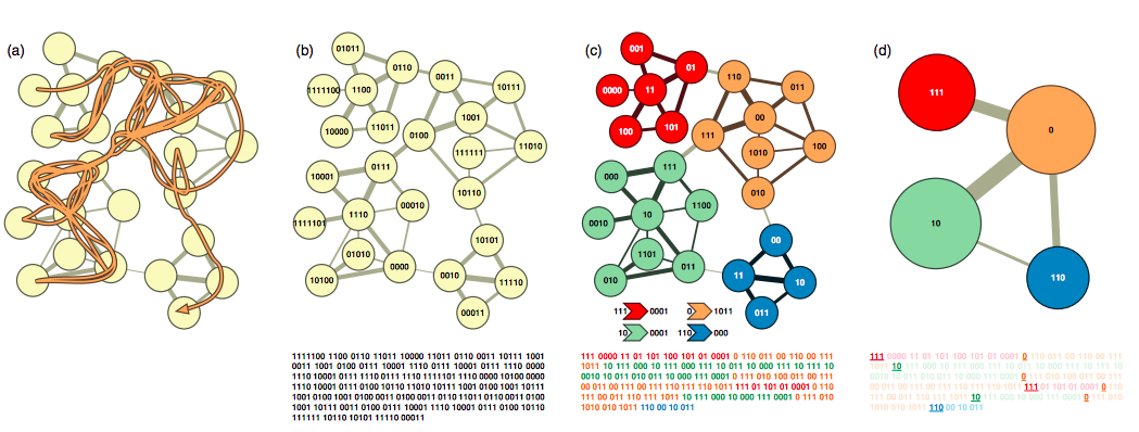InfoMap encoding and clustering process. (a) Random walk; (b) directly constructing a Huffman code based on the random-walk probabilities; (c) hierarchical encoding; (d) category encoding within hierarchical encoding. The bottom shows the corresponding encoded sequences, and it's clear that the hierarchical-encoding sequence is shorter

This is the clustering process of InfoMap — construct transition probabilities, perform a random walk on the graph to generate a sequence, then apply hierarchical encoding to that sequence and minimize the objective $\eqref{eq:loss}$, thereby completing the clustering.

Incidentally, back when DeepWalk (2014) proposed performing random walks on a graph to generate sequences and then applying Word2Vec, many people found it quite novel — a real breakthrough. But looking back now, the idea of random walks on graphs actually has a much longer history.

InfoMap

Now let's flesh out the above process in more precise, mathematical terms — after all, mathematical formulas are the only way to clearly describe the underlying principle.

First of all, we don't actually need to simulate the random walk on the graph, because in fact we don't need the generated sequence itself — we only need to know the probability of each object appearing in the sequence generated by the random walk. For this, we just need to solve the equation

\begin{equation}\begin{pmatrix}p_1\\p_2\\ \vdots \\p_n\end{pmatrix} = \begin{pmatrix}p_{1\to 1} & p_{2\to 1} & \cdots & p_{n\to 1}\\p_{1\to 2} & p_{2\to 2} & \cdots & p_{n\to 2} \\ \vdots& \vdots& \ddots & \vdots \\p_{1\to n} & p_{2\to n} & \cdots & p_{n\to n}\end{pmatrix} \begin{pmatrix}p_1\\p_2\\ \vdots \\p_n\end{pmatrix}\label{eq:pab}\end{equation}

or written as $p_{\beta}=\sum\limits_{\alpha} p_{\alpha}p_{\alpha\to\beta}$. This is easy to understand: we're assuming that the final stationary distribution is $(p_1,p_2,\cdots,p_n)$, so taking one more step of the random walk should leave it unchanged.

However, with a plain random walk like this, the result may depend on the initial value of the iteration — in other words, the solution to the equation $\eqref{eq:pab}$ may not be unique. This isn't hard to imagine: if the graph has some isolated regions, then a walk that wanders into such an isolated region can never leave it, so the probability of all nodes outside that region ends up being 0. Having the result depend on the initial value is unreasonable — the clustering result should depend only on the graph itself. To solve this problem, the author introduces a "teleportation probability" $\tau$: with probability $1-\tau$ we follow the transition probabilities $p_{\beta\to\alpha}$ to random-walk as usual, and with probability $\tau$ we jump to a uniformly random node in the graph. In that case, the equation above becomes

\begin{equation}p_{\beta}=(1-\tau)\sum_{\alpha} p_{\alpha}p_{\alpha\to\beta} + \tau \sum_{\alpha} \frac{p_{\alpha}}{n}\label{eq:pa}\end{equation}

which is equivalent to replacing the transition probability $p_{\alpha\to\beta}$ with $(1-\tau)p_{\alpha\to\beta} + \tau/n$.

With this teleportation probability, the model generally won't get trapped in some local solution, thereby giving a unique solution. $\tau$ is an extra hyperparameter, which the author sets to $\tau=0.15$; and to make the result more robust to $\tau$, the author uses several additional techniques — for the details, please refer to the author's papers The map equation and Community detection and visualization of networks with the map equation framework.

Now that we have $p_{\alpha}$, to reach our objective $\eqref{eq:loss}$ we're still missing $q_{i\curvearrowright}$: $q_{i\curvearrowright}$ is the probability of a category, i.e., the probability of the termination marker. When does the termination marker occur? The termination marker occurs when what follows is no longer in the same $i$ category — so the probability of the termination marker is really the "probability of jumping from one category to another," in other words, the probability that the event "leaving category $i$" occurs during the random walk. It equals

\begin{equation}q_{i\curvearrowright} = \sum_{\alpha\in i}\sum_{\beta\not\in i} p_{\alpha} p_{\alpha\to\beta}\end{equation}

If we include the teleportation probability, we need to replace $p_{\alpha\to\beta}$ with $(1-\tau)p_{\alpha\to\beta} + \tau/n$, giving

\begin{equation}\begin{aligned}q_{i\curvearrowright} =& \sum_{\alpha\in i}\sum_{\beta\not\in i} p_{\alpha} \left[(1-\tau)p_{\alpha\to\beta} + \frac{\tau}{n}\right]\\ =& \tau\frac{n - n_i}{n}\sum_{\alpha\in i}p_{\alpha} + (1-\tau)\sum_{\alpha\in i}\sum_{\beta\not\in i} p_{\alpha}p_{\alpha\to\beta} \end{aligned}\label{eq:q-exit}\end{equation}

where $n_i$ is the number of objects within category $i$.

Now that we have the forms of both $p_{\alpha}$ and $q_{i\curvearrowright}$, in principle we should normalize $p_{\alpha}$ and $q_{i\curvearrowright}$ according to equation $\eqref{eq:guiyi}$, but the form of $\eqref{eq:q-exit}$ shows that $q_{i\curvearrowright}$ is homogeneous in $p_{\alpha}$, and the optimization objective $\eqref{eq:loss}$ only cares about relative probabilities, so whether or not we normalize doesn't actually matter.

Alright, now that everything is in place, the whole InfoMap pipeline emerges (the search strategy in step 3 will be introduced in the experiments section):

1. Define the transition probabilities $p_{\alpha\to\beta}$ between samples;
2. Numerically solve $\eqref{eq:pa}$ to obtain $p_a$;
3. Search over clustering schemes to make $\eqref{eq:loss}$ as small as possible, where $q_{i\curvearrowright}$ under each clustering scheme is computed according to $\eqref{eq:q-exit}$.

Generalization ideas

What makes InfoMap so elegant isn't just its beautiful information-theoretic interpretation and its lack of excessive hyperparameters — it's also how easily it generalizes, at least conceptually.

For instance, so far we've been using two-level hierarchical encoding, but we could instead construct multi-level hierarchical encoding, i.e., clustering the clusters themselves. In fact, generalizing the optimization objective $\eqref{eq:loss}$ from two levels to multiple levels is tedious but technically straightforward, since we just need to mimic the two-level encoding scheme and work out the corresponding multi-level encoding scheme (introducing category-within-category labels and termination markers, etc.). For the details, see Multilevel compression of random walks on networks reveals hierarchical organization in large integrated systems and Community detection and visualization of networks with the map equation framework; we won't go into further detail here.

Another example is generalizing to overlapping community detection. Overlapping community detection means that a single object may belong to several different categories simultaneously. The article What Is Community Detection? gives a vivid example about neighborhood aunties forming square-dancing teams: generally, when an auntie joins an activity, she'll preferentially choose the dance team from her own neighborhood. But some aunties have more energy and find it unsatisfying to only join their own neighborhood's team, or they're the sociable type who wants to make more friends through square dancing — so they might join several dance teams from neighboring communities at once. In other words, she belongs to multiple communities (categories) simultaneously. From an NLP word-clustering perspective, overlapping community detection corresponds to discovering polysemous words. For InfoMap, mining overlapping communities still amounts to minimizing $\eqref{eq:loss}$: assigning the same object to multiple categories introduces some redundancy into the encoding of that object itself, but it may reduce the use of category labels and termination markers, thereby lowering the overall average code length. For the paper, see Compression of Flow Can Reveal Overlapping-Module Organization in Networks.

These generalization properties are things that most other clustering algorithms and community-detection algorithms lack, which further highlights how powerful and elegant InfoMap is. In addition, the publications page on the official website has a whole pile of papers on InfoMap extensions and applications, well worth checking out:

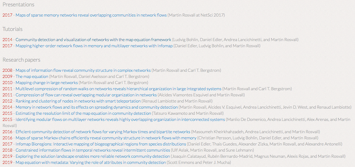List of papers provided on InfoMap's official website

Experiments

Alright, enough theory for now — time to get our hands dirty with some experiments. This section will first briefly introduce how InfoMap actually searches for a clustering strategy, and then give an example of word clustering, to get an initial feel for InfoMap's charm.

Solution algorithm

InfoMap's earliest solving algorithm was greedy search plus simulated annealing. In the greedy search, every node starts out as its own separate category; then the two categories whose merger produces the largest decrease in $\eqref{eq:loss}$ are merged into one, and this process is repeated until no further decrease is possible. Simulated annealing is then used to fine-tune the clustering scheme found by the greedy search. (From Maps of random walks on complex networks reveal community structure.)

Later, in The map equation, the author improved the greedy search and removed the simulated annealing step, striking a balance between speed and quality. The improved algorithm goes roughly as follows (again, see the original paper for details):

1. Initialize each node as its own separate category;
2. Traverse the nodes in random order, assigning each node to whichever neighboring category produces the largest decrease in $\eqref{eq:loss}$;
3. Repeat step 2 (using a different random order each time) until $\eqref{eq:loss}$ no longer decreases;
4. Apply some additional strategies to fine-tune the clustering result obtained from the previous three steps.

Whether we're talking about the early solving algorithm or the later improved one, InfoMap can solve things remarkably fast. The paper gives two sets of reference results: 1) plain greedy search successfully completed community detection on a graph with 2.6 million nodes and 29 million edges; 2) the improved algorithm completed community detection on a graph with 10,000 nodes and 100,000 edges in under 5 seconds (and given how much slower computers were back then, running it today would take even less time).

Installation notes

The authors implemented InfoMap in C++, and provide interfaces for third-party languages such as Python and R, with support for Linux, Mac OS X, and Windows.

Official site: https://www.mapequation.org/code.html

Github: https://github.com/mapequation/infomap

Here we're naturally only concerned with the Python interface. After some fiddling around, I've established the following:

1. InfoMap currently has two versions: the 0.x series is the stable release, while 1.0 is in beta;
2. Installing directly via pip install infomap gives you the beta 1.0 version, but it's missing some functionality and only supports Python 3.x;
3. The fully-featured version is still 0.x, which supports Python 2.7 — but for some reason, after successfully compiling the latest 0.x version, import throws an error.

Since I had previously installed InfoMap and used it quite comfortably, but ran into all sorts of issues with the newer version (I have no idea what the authors changed), I'd suggest pulling an older 0.x release from Github and compiling it manually. Here's some reference code for compiling and installing:

wget -c https://github.com/mapequation/infomap/archive/6ab17f8b18a6fdf34b2a53454f79a3b976a49201.zip
unzip 6ab17f8b18a6fdf34b2a53454f79a3b976a49201.zip
cd infomap-6ab17f8b18a6fdf34b2a53454f79a3b976a49201
cd examples/python
make

# 编译完之后，当前目录下就会有一个infomap文件夹，就是编译好的模块；
# 为了方便调用，可以复制到python的模块文件夹（每台电脑的路径可能不一样）中
python example-simple.py
cp infomap /home/you/you/python/lib/python2.7/site-packages -rf

The examples/python folder provides some simple demos you can refer to.

Word clustering

Below, we pair InfoMap with Word2Vec to run a word-clustering example. The code is located at:

https://github.com/bojone/infomap/blob/master/word_cluster.py

Clustering results (partial):

[u'妹妹', u'姐姐', u'哥哥', u'弟弟', u'爸爸', u'儿子', u'母亲', u'女儿', u'父亲', u'妻子', u'爷爷', u'老婆', u'丈夫', u'男友', u'女友', u'爱人', u'妈妈', u'长子', u'小时候', u'父母', u'祖父', u'情人', u'亲人', u'弟', u'家人', u'夫妇', u'妻', u'兄', u'妹', u'家里', u'姐妹', u'父', u'嫁给', u'从小', u'子女', u'嫁', u'夫', u'家中', u'娶', u'姐', u'叔', u'长大', u'夫人', u'父子', u'在家', u'娘', u'兄弟', u'家属', u'奴', u'母', u'子', u'哥', u'儿', u'儿女', u'小姐'] (family-relation terms such as younger sister, older sister, older brother, younger brother, father, son, mother, daughter, wife, husband, boyfriend, girlfriend, grandfather, etc.)
[u'加强', u'建立健全', u'推进', u'拟定', u'落实', u'提高', u'规章制度', u'会同', u'搞好', u'切实', u'负责', u'促进', u'贯彻落实', u'制订', u'增强', u'抓好', u'深化', u'组织协调', u'拟订', u'加快', u'加大', u'实施', u'着力', u'有利于', u'制定', u'推动', u'进一步', u'贯彻', u'督促', u'改善', u'大力', u'贯彻执行', u'充分发挥', u'牵头', u'政策措施', u'年度计划', u'强化', u'提升', u'增进', u'中长期', u'健全', u'优化', u'方针', u'做好', u'协调', u'统筹', u'承办', u'协助', u'全力', u'积极', u'责任制', u'党和国家', u'步伐', u'力度', u'承担', u'开展', u'巩固', u'编制', u'有利', u'改进', u'加深', u'不利', u'各项', u'加速', u'围绕', u'组织', u'衔接', u'认真'] (bureaucratic/policy-implementation vocabulary such as strengthen, establish and improve, advance, formulate, implement, improve, regulations, coordinate, etc.)
[u'股权', u'证券', u'融资', u'股票', u'金融机构', u'上市公司', u'信贷', u'债券', u'商业银行', u'贷款', u'金融', u'期货', u'信托', u'存款', u'债权', u'担保', u'股份', u'银行', u'抵押', u'董事长', u'副总经理', u'外汇', u'总经理', u'利率', u'董事', u'余额', u'总监', u'保险公司', u'并购', u'股东', u'利息', u'CEO', u'国有企业', u'债务', u'资产', u'分行', u'经理', u'负债', u'股市', u'信用', u'总额', u'总裁', u'国有资产', u'股价', u'投资者', u'资本', u'汇率', u'数额', u'金额', u'投资', u'首席', u'账户', u'国有', u'货币', u'邮政', u'董事会', u'创始人', u'改制', u'支行', u'主管', u'出资', u'破产', u'重组', u'财产', u'披露', u'固定资产', u'收购', u'上涨', u'财富', u'商业', u'现金'] (financial/business terms such as equity, securities, financing, stocks, financial institutions, listed companies, credit, bonds, commercial banks, loans, etc.)
[u'教师', u'教学', u'教研', u'素质教育', u'课堂教学', u'教学质量', u'教学改革', u'该校', u'学生', u'基础教育', u'我校', u'高职', u'德育', u'教职工', u'职业教育', u'高等院校', u'办学', u'教师队伍', u'院校', u'师资', u'在校生', u'考生', u'教育', u'高等学校', u'同学们', u'专任教师', u'毕业生', u'班级', u'班主任', u'报考', u'人才培养', u'高等教育', u'在校', u'孩子们', u'高校', u'老师', u'学员', u'招生', u'全校', u'育人', u'学子', u'大学生', u'教学班', u'校长', u'入学', u'家长', u'在校学生', u'录取', u'师生', u'青少年', u'同学', u'全日制', u'心理健康', u'招收', u'课堂', u'报名', u'青年', u'校友', u'先生', u'义务教育', u'校园', u'校', u'成绩', u'女士'] (education-related terms such as teacher, teaching, teaching research, quality education, classroom instruction, teaching quality, students, basic education, etc.)
[u'慢性', u'疾病', u'糖尿病', u'急性', u'病变', u'肿瘤', u'高血压', u'治疗', u'炎症', u'并发症', u'心脏病', u'癌症', u'水肿', u'患者', u'病理', u'病因', u'腹泻', u'呕吐', u'咳嗽', u'症状', u'便秘', u'临床表现', u'出血', u'病人', u'症', u'贫血', u'手术', u'头痛', u'病例', u'疗效', u'康复', u'发病', u'综合征', u'疗法', u'诊断', u'发作', u'切除', u'病情', u'功效', u'损伤', u'病', u'传染病', u'鉴别', u'感染', u'患', u'病毒', u'瘤', u'术', u'囊', u'畸形', u'部位', u'发热', u'伴有', u'中毒'] (medical terms such as chronic, disease, diabetes, acute, lesion, tumor, hypertension, treatment, inflammation, complications, heart disease, cancer, etc.)
[u'魔王', u'恶魔', u'妖', u'魔', u'冥', u'邪恶', u'吸血鬼', u'怪物', u'死神', u'鬼', u'幽灵', u'猎人', u'幻', u'魔兽', u'仙', u'黑暗', u'诅咒', u'封印', u'僵尸', u'毁灭', u'舰', u'舰队', u'玄', u'咒', u'精灵', u'幽', u'兽', u'艘', u'魔鬼', u'凶', u'骑士', u'BOSS', u'地狱', u'复活', u'国王', u'公主', u'女王', u'神仙', u'仙人', u'诀', u'召唤', u'尸', u'逍遥', u'魔法', u'怪', u'法术', u'神', u'王子', u'女神', u'魔力', u'灵', u'勇士', u'魂', u'邪', u'天使', u'怪兽', u'化身', u'尸体', u'武士', u'海盗', u'恶', u'戒', u'预言', u'死者', u'风流', u'光明', u'副本', u'变身', u'丹', u'杀手', u'正义', u'武功', u'荒'] (fantasy/gaming terms such as demon king, devil, monster, vampire, ghost, hunter, dark, curse, seal, zombie, destruction, fleet, elf, knight, boss, hell, resurrection, king, princess, queen, immortal, etc.)

Clearly, the clustering results look quite good.

Summary

It took me several days, but I've finally finished this blog post — an algorithm I'd shelved for over two years, and I've now finally picked it back up and gotten a solid understanding of it.

To sum up, InfoMap is a clustering/community-detection algorithm built on top of transition probabilities, with a clean information-theoretic interpretation (the minimum-entropy interpretation), and it has almost no hyperparameters to speak of (or rather, its only "hyperparameter" is how you construct the transition probabilities). These days quite a few fields are starting to pay attention to it, trying to use it to mine data for modules with meaningful internal connections (and really, which field doesn't have some structure of nodes and graph networks lurking in it?). My advisor originally suggested I use it to analyze genomic data — unfortunately I never actually got that project to completion. Regardless, it's such an elegant and beautiful method that I think it deserves to be properly understood.

Finally, as a side note: this is already the fifth article in the minimum entropy principle series. How far can it still go? Let's wait and see.