A Brief Introduction to the Non-Adversarial Generative Model GLANN

非对抗式生成模型GLANN的简单介绍 苏剑林 · 2019-02-26 · Machine Learning probability generative model

A while back I noticed that Facebook had published a non-adversarial generative model called GLANN (posted on arXiv last December), claiming that it could generate 1024-resolution high-definition faces without any adversarial training. This piqued my interest, so I read through it, and indeed came away with some takeaways — but also a bit disappointed. As for why disappointed, that will become clear as you read on.

Original paper: Non-Adversarial Image Synthesis with Generative Latent Nearest Neighbors

Introduction from Synced (机器之心): Why Let GANs Have All the Fun? Facebook Proposes a Non-Adversarial Generation Method, GLANN

Example results:

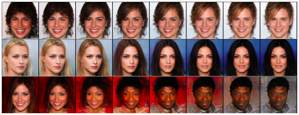GLANN example results more

Below is a simple walkthrough of the ideas behind the GLANN model.

Implicit Maximum Likelihood

The foundation of the whole GLANN method is "Implicit Maximum Likelihood Estimation," from the paper Implicit Maximum Likelihood Estimation, abbreviated as "IMLE." This paper only appeared on arXiv last September, which honestly surprised me quite a bit — because the algorithm is extremely simple, and I had already been using it two years earlier. I always assumed it was an obviously valid method, yet it took this long for someone to actually write it up as a paper... (feels like I missed out on tens of millions in potential recognition)

Directly Estimating the Probability Distribution

The appendix of the IMLE paper gives a long and complicated mathematical derivation, but in my opinion that's really not necessary. IMLE is essentially just the result of approximating an integral over a Dirac distribution.

In general, the following sampling process:

\begin{equation}z\sim q(z),\quad x = G(z)\end{equation}

is actually equivalent to assuming that the distribution of $x$ is

\begin{equation}q(x)=\int \delta\big(x-G(z)\big)q(z)dz\end{equation}

where $q(z)$ is generally taken to be a normal or uniform distribution, and $\delta(\cdot)$ represents the (multivariate) Dirac delta function.

Note that $q(x)$ can also be written as

\begin{equation}q(x)=\mathbb{E}_{z\sim q(z)}\big[\delta\big(x-G(z)\big)\big]\end{equation}

and $\delta(\cdot)$ is in fact just a Gaussian distribution whose variance tends to zero:

\begin{equation}\delta(x)=\lim_{\sigma\to 0}\frac{1}{(2\pi\sigma^2)^{d/2}}\exp\left(-\frac{\Vert x\Vert^2}{2\sigma^2}\right)\end{equation}

Given this, we might as well let $\sigma$ take some finite value, compute everything, and only then let $\sigma\to 0$, i.e.

\begin{equation}q(x)=\lim_{\sigma\to 0}\mathbb{E}_{z\sim q(z)}\left[\frac{1}{(2\pi\sigma^2)^{d/2}}\exp\left(-\frac{\Vert x - G(z)\Vert^2}{2\sigma^2}\right)\right]\end{equation}

Then we perform maximum likelihood estimation, taking $-\int p(x)\log q(x)dx$ as the loss, where $p(x)$ is the distribution of the real samples:

\begin{equation}\begin{aligned}loss=&-\int p(x)\log \left\{\mathbb{E}_{z\sim q(z)}\left[\frac{1}{(2\pi\sigma^2)^{d/2}}\exp\left(-\frac{\Vert x - G(z)\Vert^2}{2\sigma^2}\right)\right]\right\}dx\\ =&\mathbb{E}_{x\sim p(x)}\left[-\log \left\{\mathbb{E}_{z\sim q(z)}\left[\frac{1}{(2\pi\sigma^2)^{d/2}}\exp\left(-\frac{\Vert x - G(z)\Vert^2}{2\sigma^2}\right)\right]\right\}\right]\\ \sim &\mathbb{E}_{x\sim p(x)}\left[-\log \left\{\mathbb{E}_{z\sim q(z)}\left[\exp\left(-\frac{\Vert x - G(z)\Vert^2}{2\sigma^2}\right)\right]\right\}\right]\end{aligned}\end{equation}

In this last expression we have already dropped the constant that is irrelevant to the optimization.

Now let's turn $\mathbb{E}$ into a sampling process, i.e. substitute $x_1,x_2,\dots,x_M\sim p(x)$ and $z_1,z_2,\dots,z_N\sim q(z)$ into the loss:

\begin{equation}\begin{aligned}loss\sim& -\frac{1}{M}\sum_{i=1}^M \log \left\{\frac{1}{N}\sum_{j=1}^N\exp\left(-\frac{\Vert x_i - G(z_j)\Vert^2}{2\sigma^2}\right)\right\}\\ \sim& -\frac{1}{M}\sum_{i=1}^M \log \left\{\sum_{j=1}^N\exp\left(-\frac{\Vert x_i - G(z_j)\Vert^2}{2\sigma^2}\right)\right\}\end{aligned}\end{equation}

From the article Seeking a Smooth Maximum Function we know that $\text{logsumexp}$ (exponentiate, sum, then take the log) is actually a smooth approximation to $\max$; when $\sigma\to 0$ it becomes exactly $\max$, and with a minus sign in front this is $\min$. So the simplest form when $\sigma\to 0$ is:

\begin{equation}loss\sim \frac{1}{M}\sum_{i=1}^M \left(\min_{j=1}^N \Vert x_i - G(z_j)\Vert^2\right)\end{equation}

This is exactly the loss used by IMLE. (The derivation above is a bit long only because I wrote it out in detail — it's really not hard.)

So, concretely, the IMLE procedure is:

1. Sample a batch of real samples $x_1,x_2,\dots,x_M$;
2. Sample a batch of noise $z_1,z_2,\dots,z_N$, obtaining a batch of fake samples $\hat{x}_1,\hat{x}_2,\dots,\hat{x}_N$;
3. For each real sample $x_i$, find its nearest fake sample $\hat{x}_{\rho(i)}$;
4. Minimize the average distance $\frac{1}{M}\sum\limits_{i=1}^M \Vert x_i - \hat{x}_{\rho(i)}\Vert^2$.

Analysis and Discussion of the Results

Setting the derivation aside, this algorithm is really quite intuitive: if every real sample can find a sufficiently close match among the fake samples, doesn't that mean the fake samples are pretty good too? So it really is baffling to me that this algorithm took so long to be written up as a paper.

Now let's look at the results. There's nothing wrong with the principle behind the algorithm, but the problem is that "closest" above is measured using L2 distance, and L2 is not a great distance metric for images. So it's not surprising that this method suffers from the same blurriness issue as VAEs. In fact, if you look at the results on CelebA, it doesn't even match VAE:

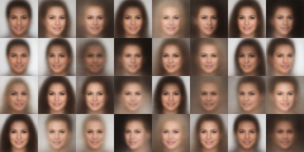IMLE results on CelebA

Code: https://github.com/bojone/gan/blob/master/imle.py

Actually, this idea can also be generalized to divergence optimization in general. For example, we could use

\begin{equation}KL(q(x)\Vert p(x))=\int q(x)\log \frac{q(x)}{p(x)}dx=\mathbb{E}_{x\sim q(x)}\big[\log q(x)-\log p(x)\big]\end{equation}

as the optimization objective, and process $\log q(x)、\log p(x)$ in the same way. Then the result becomes:

\begin{equation}loss\sim -\frac{1}{M}\sum_{i=1}^M \left(\min_{j=1}^N \Vert G(z_i) - x_j\Vert^2 - \min_{j=1}^K \Vert G(z_i) - G(z_j)\Vert^2\right)\end{equation}

Or, by introducing a margin $m$, we can get somewhat better results:

\begin{equation}loss\sim -\frac{1}{M}\sum_{i=1}^M \left(\min_{j=1}^N \Vert G(z_i) - x_j\Vert^2 + \text{relu}\left(m - \min_{j=1}^K \Vert G(z_i) - G(z_j)\Vert^2\right)\right)\end{equation}

Note that here we need to sample two separate batches of fake samples, otherwise the second term becomes meaningless (within the same batch, the second term would always be 0). The second term is there to prevent mode collapse. The procedure for this new algorithm is:

1. Sample a batch of real samples $x_1,x_2,\dots,x_M$;
2. Sample a batch of noise $z_1,z_2,\dots,z_N$, obtaining a batch of fake samples $\hat{x}_1,\hat{x}_2,\dots,\hat{x}_N$;
3. Sample another batch of noise $z_{N+1},z_{N+2},\dots,z_{N+K}$, obtaining another batch of fake samples $\hat{x}_{N+1},\hat{x}_{N+2},\dots,\hat{x}_{N+K}$;
4. For each fake sample $\hat{x}_i$ ($1\leq i\leq N$), find its nearest real sample $x_{\rho_1(i)}$;
5. For each fake sample $\hat{x}_i$ ($1\leq i\leq N$), find its nearest fake sample within $\hat{x}_{N+1},\hat{x}_{N+2},\dots,\hat{x}_{N+K}$, $x_{N+\rho_2(i)}$;
6. Minimize the "real-fake" distance while maximizing the "fake-fake" distance — that is, the loss above.

Example results:

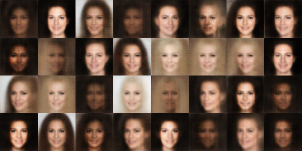Another IMLE variant's results on CelebA

They're all about the same...

From IMLE to GLANN

Coming back to IMLE itself: it's easy to imagine that the main reason IMLE performs relatively poorly is its use of L2 distance. So what if we switched to a different distance? Is there some off-the-shelf loss function that better captures image realism?

Perceptual Loss

There actually is one: perceptual loss! This perceptual loss originated from style transfer, from the paper Perceptual Losses for Real-Time Style Transfer and Super-Resolution. Computing this perceptual loss is a bit involved: it requires a pretrained ImageNet model — VGG is typically used for simplicity — from which you compute the activations of the last few hidden layers, then separately compute the L2 (or L1) distance between the hidden-layer vectors and the L2 (or L1) distance between the corresponding Gram matrices, and finally add them together.

This distance works pretty well for style transfer tasks, but it's somewhat complicated to compute, and feels more like an engineering artifact than something derived from theory, so I'm not particularly fond of it and won't go into more detail here. In short, we can combine perceptual loss with IMLE like so:

\begin{equation}loss\sim \frac{1}{M}\sum_{i=1}^M \left(\min_{j=1}^N d_{perceptual}\big(x_i,G(z_j)\big)\right)\label{eq:perceptual-1}\end{equation}

A Transitional Ingredient: GLO

Directly optimizing the objective $\eqref{eq:perceptual-1}$ is fine in theory, but computationally very expensive, because as mentioned, perceptual loss is complex to compute and requires an off-the-shelf ImageNet model. If the batch size is 64, then for every batch we'd need to compute $64^2=4096$ perceptual losses and then take the minimum — this would be unbearably slow, or might not even run at all.

So GLANN also borrows a trick called GLO, from the paper Optimizing the Latent Space of Generative Networks.

GLO is, once again, an extremely simple idea that somehow got turned into its own paper. GLO was never intended to build a generative model at all — it just aims to obtain a low-dimensional embedding. Suppose the set of real samples is $x_1,x_2,\dots,x_M$; then the optimization objective of GLO is

\begin{equation}\mathop{\text{argmin}}_{G,\hat{z}_1,\dots,\hat{z}_M}\frac{1}{M}\sum_{i=1}^M d\big(x_i, G(\hat{z}_i)\big)\quad \text{s.t.}\quad \Vert z_i\Vert=1\end{equation}

GLO directly optimizes over $\hat{z}_1,\dots,\hat{z}_M$, which is equivalent to an embedding layer, training an embedding for each image. The parts of this model that can be varied are the constraint imposed on the embeddings and the metric $d$ used. For GLANN, the metric used is perceptual loss:

\begin{equation}\mathop{\text{argmin}}_{G,\hat{z}_1,\dots,\hat{z}_M}\frac{1}{M}\sum_{i=1}^M d_{perceptual}\big(x_i, G(\hat{z}_i)\big)\quad \text{s.t.}\quad \Vert z_i\Vert=1\end{equation}

This way, even with a batch size of 64, we only need to compute 64 perceptual losses per batch, since there's no pairwise comparison involved.

The Final Result: GLANN

Now that we have $\hat{z}_1,\dots,\hat{z}_M$, $G(\hat{z}_i)$ can be used to generate images. All that remains is to treat $\hat{z}_1,\dots,\hat{z}_M$ as the "original image" and apply IMLE to it (and now we can use L2, since we're only working in latent space):

\begin{equation}\mathop{\text{argmin}}_{T}\frac{1}{M}\sum_{i=1}^M \left(\min_{j=1}^N \Vert \hat{z}_i - T(z_j)\Vert^2\right)\end{equation}

and we get our generative model. The full generation process is:

\begin{equation}z\sim q(z)\quad\xrightarrow{\quad T\quad }\quad \hat{z}_i \quad \xrightarrow{\quad G\quad }\quad x_i\end{equation}

Personal Assessment

That wraps up our walkthrough of the GLANN model. All in all, this is a model that combines a handful of tricks. As for the quality of results — just look at the images at the top of the post. Honestly, I don't think the results are particularly impressive; the backgrounds always tend to look messy. That said, it's undoubtedly better than plain IMLE or GLO, and should be much easier to train than a GAN.

The main improvement in GLANN is replacing L2 distance with perceptual loss, and I imagine this substitution could be applied to many other models as well — perhaps even to VAEs. On the other hand, the perceptual-loss approach feels too much like an engineering hack, and I don't find it particularly interesting, so I'm not motivated to dig deeper into it. Also, the GLANN paper reports an advantage in FID scores on certain datasets, which looks impressive at first glance but is actually a somewhat unfair comparison. This is because FID itself is computed using an ImageNet model, and GLANN's loss also relies on an ImageNet model — so of course GLANN's generated images will have an edge when it comes to FID.

In fact, you could just as well use FID directly as the loss, train a GLO, and then train IMLE on top of it, and end up with a generative model. Such a model would definitely achieve a very low FID — but that wouldn't really mean much, since the realism of the generated images still wouldn't be guaranteed.