RSGAN: The "Turing Test" Idea in Adversarial Models

RSGAN：对抗模型中的“图灵测试”思想 苏剑林 · 2018-10-22 · Machine Learning probability unsupervised GAN generative model

I recently came across a really interesting piece of work called "Relativistic GAN," or RSGAN for short, from the paper The relativistic discriminator: a key element missing from standard GAN, which reportedly even got a thumbs-up from Goodfellow, the founder of GANs. This paper proposes replacing the standard GAN discriminator with a relativistic discriminator, which makes the generator converge faster and makes training more stable.

Unfortunately, the paper only discusses the results from a training and experimental perspective, without a deeper analysis, which has led many people to think it's just a training trick for GANs. But in my view, RSGAN carries much deeper implications, and could even be seen as the founder of a new school of GANs. So I've decided to give a basic introduction to the RSGAN model and the ideas behind it. That said, I should point out that, aside from arriving at the same result, the way I present things here has almost no overlap with the original paper.

The "Turing Test" idea

SGAN

SGAN is just Standard GAN. Even readers who haven't done GAN research have probably heard, through various channels, the general idea behind GANs: a "counterfeiter" keeps making forgeries, trying to fool a "discriminator"; the "discriminator" keeps improving its ability to tell real from fake. The two compete with each other and improve together, until the "discriminator" can no longer tell real from fake, at which point the "counterfeiter" has succeeded and can retire.

In modeling terms, this process is implemented through alternating training: fix the generator, and train a discriminator (a binary classifier) that outputs 1 for real samples and 0 for fake ones; then fix the discriminator, and train the generator to make fake samples output as close to 1 as possible — this latter step does not involve real samples at all.

Where the problem lies

However, this modeling process seems to place overly demanding requirements on the discriminator, because the discriminator operates in isolation: when training the generator, real samples are not involved, so the discriminator must have memorized all the properties of real samples on its own, in order to be able to guide the generator toward producing more realistic samples.

In real life, this isn't how we usually go about things. As the saying goes, "no harm without comparison, no progress without harm" — we very often distinguish real from fake by direct comparison. For example, to identify a counterfeit banknote, you might need to compare it to a genuine one; to spot a knockoff phone, you just compare it to the genuine article; and so on. Similarly, if you want to make a forgery more convincing, you need to keep the genuine article beside it for constant comparison and refinement, rather than relying solely on a "memorized" version of the genuine article.

"Comparison" makes it much easier for us to tell real from fake, and hence to make better forgeries. In the field of artificial intelligence, we have the famous "Turing test": a tester interacts with both a robot and a human without knowing in advance which is which, and if the tester cannot successfully tell them apart, then the robot is deemed to possess (in some sense) human-level intelligence. The Turing test also emphasizes the importance of comparison: if, once mixed together, the robot and the human can no longer be distinguished, then the robot has succeeded.

As we'll see next, RSGAN is based precisely on this "Turing test" idea: if the discriminator cannot tell apart a mixture of real and fake images, then the generator has succeeded — and in order to generate better images, the generator also needs to make direct use of real images.

The basic RSGAN framework

Analyzing SGAN

First, let's review the standard GAN procedure. Let the real sample distribution be $\tilde{p}(x)$ and the fake sample distribution be $q(x)$. Then, with the generator fixed, we optimize the discriminator $T(x)$ as:

\begin{equation}\min_{T}-\mathbb{E}_{x\sim \tilde{p}(x)}[\log \sigma(T(x))] - \mathbb{E}_{x\sim q(x)}[\log(1-\sigma(T(x)))]\label{eq:sgan-d}\end{equation}

Here $\sigma$ is the sigmoid activation function. Then, with the discriminator fixed, we optimize the generator $G(z)$ as:

\begin{equation}\min_{G}\mathbb{E}_{x=G(z),z\sim q(z)}[h(T(x))]\label{eq:sgan-g}\end{equation}

Note that here we have an undetermined $h$, which we'll analyze shortly.

From $\eqref{eq:sgan-d}$ we can solve for the optimal discriminator, which satisfies (proof given later)

\begin{equation}\frac{\tilde{p}(x)}{q(x)}=\frac{\sigma(T(x))}{1 - \sigma(T(x))} = e^{T(x)}\end{equation}

Substituting this into $\eqref{eq:sgan-g}$, we find that the result is

\begin{equation}\min_{G}\mathbb{E}_{x=G(z),z\sim q(z)}\left[h\left(\log\frac{\tilde{p}(x)}{q(x)}\right)\right]=\min_{G}\int q(x)\left[h\left(\log\frac{\tilde{p}(x)}{q(x)}\right)\right]dx \end{equation}

I've written the last equality this way because, by simply setting $f(t)=h(\log(t))$, we can see that it takes the form of an f-divergence. That is, minimizing $\eqref{eq:sgan-g}$ is equivalent to minimizing the corresponding f-divergence. For more on f-divergences, see my earlier post A Brief Introduction to f-GAN: The GAN Model Factory. The essential requirement on f in an f-divergence is that $f$ be a convex function, so we only need to choose $h$ such that $h(\log(t))$ is convex. The simplest case is $h(t)=-t$, for which $h(\log(t))=-\log t$ is convex, and in this case $\eqref{eq:sgan-g}$ becomes

\begin{equation}\min_{G}\mathbb{E}_{x=G(z),z\sim q(z)}[-T(x)]\end{equation}

There are many similar choices; for instance, when $h(t)=-\log \sigma(t)$, $h(\log(t))=\log \left(1+\frac{1}{t}\right)$ is also convex (for $t > 0$), so

\begin{equation}\min_{G}\mathbb{E}_{x=G(z),z\sim q(z)}[-\log\sigma(T(x))]\end{equation}

is also a reasonable choice, and it happens to be one of the commonly used generator losses in GANs. There are similar choices such as $h(t)=\log(1-\sigma(t))$, which I won't enumerate here.

The RSGAN objective

Here, let's directly state the RSGAN optimization objective: with the generator fixed, we optimize the discriminator $T(x)$ as:

\begin{equation}\min_{T}-\mathbb{E}_{x_r\sim \tilde{p}(x), x_f\sim q(x)}[\log \sigma(T(x_r)-T(x_f))]\label{eq:rsgan-d}\end{equation}

Here $\sigma$ is again the sigmoid activation function. Then, with the discriminator fixed, we optimize the generator $G(z)$ as:

\begin{equation}\min_{G}\mathbb{E}_{x_r\sim \tilde{p}(x), x_f=G(z),z\sim q(z)}[h(T(x_f) - T(x_r))]\label{eq:rsgan-g}\end{equation}

As with SGAN, we've kept a general $h$ here, with the same requirement on $h$ as discussed above for SGAN. The choice made in the original RSGAN paper is

\begin{equation}\min_{G}-\mathbb{E}_{x_r\sim \tilde{p}(x), x_f=G(z),z\sim q(z)}[\log\sigma(T(x_f) - T(x_r))]\end{equation}

This looks like it simply replaces the two terms of the SGAN discriminator with a single relativistic discriminator. So what changes in the corresponding analytical results?

Theoretical results

Using the calculus of variations (proof given later), we can show that the optimal solution for $\eqref{eq:rsgan-d}$ is

\begin{equation}\frac{\tilde{p}(x_r)q(x_f)}{\tilde{p}(x_f)q(x_r)}=\frac{\sigma(T(x_r)-T(x_f))}{\sigma(T(x_f)-T(x_r))}=e^{T(x_r)-T(x_f)}\end{equation}

Substituting this into $\eqref{eq:rsgan-g}$, the result is

\begin{equation}\begin{aligned}&\min_{G}\mathbb{E}_{x_r\sim \tilde{p}(x), x_f=G(z),z\sim q(z)}\left[h\left(\log\frac{\tilde{p}(x_f)q(x_r)}{\tilde{p}(x_r)q(x_f)}\right)\right]\\ =&\min_{G}\iint \tilde{p}(x_r)q(x_f)\left[h\left(\log\frac{\tilde{p}(x_f)q(x_r)}{\tilde{p}(x_r)q(x_f)}\right)\right] dx_r dx_f\end{aligned}\label{eq:rsgan-gg}\end{equation}

This result is the real heart of RSGAN: it optimizes the f-divergence between $\tilde{p}(x_r)q(x_f)$ and $\tilde{p}(x_f)q(x_r)$!

What does this mean? It means: suppose we sample a real point $x_r$ and a fake point $x_f$, and then swap them — treating the fake one as real and the real one as fake. Can we still tell them apart? In other words, does $\tilde{p}(x_f)q(x_r)$ change much?

If there's no significant change, that means real and fake samples can no longer be distinguished, and training has succeeded; if they can still be told apart, it means we still need to use real samples to further improve the fake ones. So Equation $\eqref{eq:rsgan-gg}$ embodies precisely the "Turing test" idea in RSGAN: after shuffling the data, can it still be told apart?

Analysis of the model's effectiveness

The authors of the original paper also proposed RaSGAN, where "a" stands for "average" — using the average over the whole batch in place of a single real/fake sample. I don't think this is a particularly elegant approach, and the paper itself shows that RaSGAN's performance is not always better than RSGAN's, so I won't go into it here; interested readers can consult the original paper.

As for effectiveness, the results tables in the paper show that RSGAN improves generation quality on quite a few tasks, though not always — on average there's a slight improvement. What the authors particularly emphasize is that RSGAN speeds up training of the generator. I've also experimented with this myself, and found it faster than both SGAN and SNGAN.

My reference code:

https://github.com/bojone/gan/blob/master/keras/rsgan_sn_celeba.py

Borrowing a figure from MingtaoGuo to compare RSGAN's convergence speed:

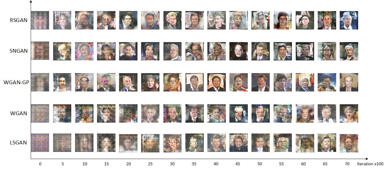RSGAN convergence speed comparison

Intuitively, RSGAN is faster because, when training the generator, it also makes use of information from real samples, rather than relying solely on the discriminator's "memory." Theoretically, by taking the difference between $T(x_r)$ and $T(x_f)$, the discriminator ends up depending only on their relative value, which conveniently corrects for whatever bias the discriminator $T$ might otherwise have, resulting in more stable gradients. I even suspect (though I haven't carefully verified this) that bringing real samples into the generator's training might improve the diversity of the fake samples, since with various real samples available for comparison, a model that only generates a single kind of sample would struggle to meet the discriminator's comparative criterion.

Related discussion

A brief summary

Overall, I think RSGAN represents a change in the underlying idea behind GANs, something perhaps even its own authors did not fully notice.

We often say that WGAN was a major breakthrough after GAN, and that's true — but it was a theoretical breakthrough, while conceptually it's the same story: reducing the distance between two distributions. It's just that the JS divergence used previously had various issues, and WGAN switched to the Wasserstein distance instead. I feel that RSGAN is more like a conceptual breakthrough — reframing things as discrimination after real and fake samples have been mixed together — even though the improvement in practice may not be dramatic. (Of course, if you want to say that in the end everyone's just pulling the two distributions closer together, I have no rebuttal to that ^_^)

Some of RSGAN's improvements are easy to reproduce. Of course, since it doesn't improve every single task, some people criticize it as just another GAN training trick. Opinions on this vary, but that doesn't stop me from appreciating and studying this paper.

By the way, the author, Alexia Jolicoeur-Martineau, is a female biostatistician at the Jewish General Hospital, and the results in the paper were obtained using just a single GTX 1060 (source here). Suddenly I feel rather proud of owning a 1060 myself... (except that while I have a 1060, I don't have a paper to show for it~)

Further musings

Finally, let me ramble a bit about some extended topics.

First, it's worth noting that WGAN's discriminator loss is itself already a difference of two terms — meaning WGAN's discriminator is already a kind of relativistic discriminator, which the authors believe is an important reason for WGAN's good performance.

Seen this way, WGAN and RSGAN already have some overlap. But I have a further thought: could the comparison based on $\tilde{p}(x_r)q(x_f)$ and $\tilde{p}(x_f)q(x_r)$ be entirely replaced with the Wasserstein distance? We know that WGAN's generator training objective is also unrelated to real samples — so how could real-sample information be better incorporated into the WGAN generator's training?

There's another question too: currently the difference being taken is just between the discriminator's final scalar outputs — could it instead be a difference between some hidden layer's representations, followed by computing an MSE or feeding it through a few more neural network layers? In any case, I feel there's still more to be done with this model...

Supplementary proofs

1. The optimal solution for $\eqref{eq:sgan-d}$
\begin{equation}\begin{aligned}&-\mathbb{E}_{x\sim \tilde{p}(x)}[\log \sigma(T(x))] - \mathbb{E}_{x\sim q(x)}[\log(1-\sigma(T(x)))]\\ > =&-\int \Big(\tilde{p}(x) \log \sigma(T(x)) + q(x) \log(1-\sigma(T(x))) \Big)dx\end{aligned}\end{equation}
Using $\delta$ to denote the variation, essentially the same as a differential:
\begin{equation}\begin{aligned}&\delta \int \Big(\tilde{p}(x) \log \sigma(T(x)) + q(x) \log(1-\sigma(T(x))) \Big)dx\\ > =& \int \left(\tilde{p}(x) \frac{\delta \sigma(T(x))}{\sigma(T(x))} + q(x) \frac{-\delta \sigma(T(x))}{1-\sigma(T(x))} \right)dx\\ > =& \int \left(\tilde{p}(x) \frac{1}{\sigma(T(x))} - q(x) \frac{1}{1-\sigma(T(x))} \right)\delta \sigma(T(x)) dx > \end{aligned}\end{equation}
The extremum is attained when the variation vanishes, and since $\delta \sigma(T(x))$ represents an arbitrary increment, if the above expression is identically zero, it means the term inside the brackets must be identically zero, i.e.
\begin{equation}\tilde{p}(x) \frac{1}{\sigma(T(x))} = q(x) \frac{1}{1-\sigma(T(x))}\end{equation}
2. The optimal solution for $\eqref{eq:rsgan-d}$
\begin{equation}\begin{aligned}&-\mathbb{E}_{x_r\sim \tilde{p}(x), x_f\sim q(x)}[\log \sigma(T(x_r)-T(x_f))]\\ > =&-\iint \tilde{p}(x_r)q(x_f)\log \sigma(T(x_r)-T(x_f)) dx_r dx_f\end{aligned}\end{equation}
Taking the variation of the above:
\begin{equation}\begin{aligned}&\delta \iint \tilde{p}(x_r)q(x_f)\log \sigma(T(x_r)-T(x_f)) dx_r dx_f\\ > =& \iint \tilde{p}(x_r)q(x_f)\frac{\delta \sigma(T(x_r)-T(x_f))}{\sigma(T(x_r)-T(x_f))} dx_r dx_f\quad[\text{next use}\sigma'(x)=\sigma(x)\sigma(-x)]\\ > =& \iint \tilde{p}(x_r)q(x_f)\sigma(T(x_f)-T(x_r)) \times (\delta T(x_r)-\delta T(x_f)) dx_r dx_f\\ > =& \iint \tilde{p}(x_r)q(x_f)\sigma(T(x_f)-T(x_r)) \delta T(x_r) dx_r dx_f \quad[\text{next swap the second term's}x_r,x_f]\\ > &\qquad - \iint \tilde{p}(x_r)q(x_f)\sigma(T(x_f)-T(x_r)) \delta T(x_f) dx_r dx_f\\ > =& \iint \tilde{p}(x_r)q(x_f)\sigma(T(x_f)-T(x_r)) \delta T(x_r) dx_r dx_f \\ > &\qquad - \iint \tilde{p}(x_f)q(x_r)\sigma(T(x_r)-T(x_f)) \delta T(x_r) dx_f dx_r\\ > =& \iint \Big[\tilde{p}(x_r)q(x_f)\sigma(T(x_f)-T(x_r)) \\ > &\qquad\qquad- \tilde{p}(x_f)q(x_r)\sigma(T(x_r)-T(x_f))\Big] \delta T(x_r) dx_r dx_f > \end{aligned}\end{equation}
The extremum is attained when the variation vanishes, so the term inside the brackets must be identically zero, i.e.
\begin{equation}\tilde{p}(x_r)q(x_f)\sigma(T(x_f)-T(x_r))=\tilde{p}(x_f)q(x_r)\sigma(T(x_r)-T(x_f))\end{equation}