Thin Water, Long Flow: f-VAEs, the Marriage of Glow and VAEs
This post is the Chinese-language version of a paper we recently posted to arXiv a few days ago. In this paper, we present an approach for combining flow-based models (such as the Glow model introduced earlier) with variational autoencoders, which we call f-VAEs. We prove theoretically that f-VAEs form a more general framework encompassing both flow-based models and variational autoencoders, and experiments show that, compared to the original Glow model, f-VAEs converge faster and achieve comparable generation quality with a much smaller network.
Original paper: f-VAEs: Improve VAEs with Conditional Flows]
Recently, generative models have attracted a great deal of attention. Among them, variational autoencoders (VAEs)] and flow-based models] are two kinds of generative models distinct from generative adversarial networks (GANs), and both have been widely studied. However, each has its own strengths and weaknesses, and this article attempts to combine them.
 ]
]
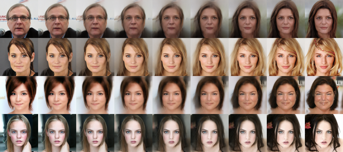
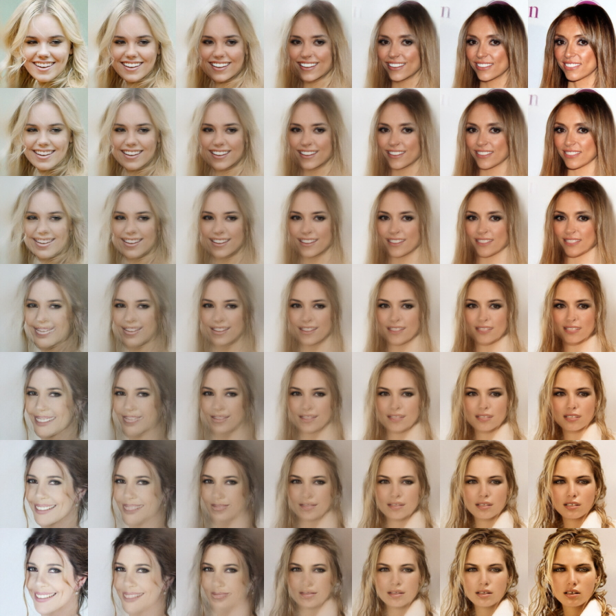
Linear interpolation between two real samples realized by f-VAEs
Basics #]
Given a dataset whose evidence distribution is $\tilde{p}(x)$, the basic idea of generative models is to fit the dataset's distribution using a form such as
$$\begin{equation}q(x)=\int q(z)q(x|z) dz\end{equation}$$
where $q(z)$ is generally taken to be a standard Gaussian distribution, and $q(x|z)$ is generally taken to be a Gaussian distribution (in VAEs) or a Dirac distribution (in GANs and flow-based models). Ideally, the optimization is done by maximizing the likelihood function $\mathbb{E}[\log q(x)]$, or equivalently, minimizing $KL(\tilde{p}(x)\Vert q(x))$. Since the integral may be intractable to compute explicitly, some special tricks are required, and this is what has led to the various different generative models. VAEs, for instance, introduce a posterior distribution $p(z|x)$ and change the optimization objective into a more tractable upper bound $KL(\tilde{p}(x)p(z|x)\Vert q(z)q(x|z))$. As is well known, VAEs enjoy fast convergence and stable training, but the images they generate tend to be blurry; we'll discuss the reason for this a bit later. In flow-based models, $q(x|z)=\delta(x - G(z))$, and $G(z)$ is carefully designed (as a composition of flows) so that this integral can be computed directly. The main building block of flow-based models is the "coupling layer": first partition $x$ into two parts $x_1,x_2$, then perform the following operation
$$\begin{equation}\begin{aligned}&y_1 = x_1\\ &y_2 = s(x_1)\otimes x_2 + t(x_1) \end{aligned}\label{eq:coupling}\end{equation}$$
This transformation is invertible, with inverse
$$\begin{equation}\begin{aligned}&x_1 = y_1\\ &x_2 = (y_2 - t(y_1)) / s(x_1) \end{aligned}\end{equation}$$
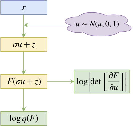
Its Jacobian determinant is $\prod_i s_i(x_i)$. This kind of transform is usually called an "affine coupling" (if $s(x_1)\equiv 1$, it's usually called an "additive coupling"), denoted $f$. By composing many coupling layers, we can obtain complex nonlinear transforms, i.e. $G = f_1 \circ f_2 \circ \dots \circ f_n$, which is what's called an "(unconditional) flow." Since the integral is computed exactly, flow-based models can directly perform maximum-likelihood optimization. The recently released Glow model demonstrated strong generative capabilities and attracted a great deal of discussion and attention. But flow-based models are generally quite large and take a long time to train (the 256x256 image generation model, for example, was trained for a week on 40 GPUs, see here] and here]), which is clearly not very friendly to work with.
Analysis #]
There are many explanations for why VAEs produce blurry images: some attribute it to the MSE loss, others to some inherent property of the KL divergence. But note one thing: even if we remove the KL-divergence term on the latent variable, turning the model into an ordinary autoencoder, the reconstructed images are still typically blurry. This suggests that the blurriness of VAE-generated images may be an inherent problem of reconstructing the original image from a low-dimensional representation. What if we set the latent dimension to be as large as the input dimension? That still doesn't seem to be enough, because standard VAEs also assume the posterior distribution to be Gaussian, which limits the model's expressive power: the family of Gaussian distributions is only a tiny fraction of all possible posterior distributions, and if the true posterior differs greatly from Gaussian, the fit will be poor.
So what's the problem with flow-based models like Glow? Flow-based models design an invertible (strongly nonlinear) transform that maps the input distribution to a Gaussian distribution. In doing so, one must guarantee not only invertibility but also that the Jacobian determinant is easy to compute, which is what leads to the design of "additive coupling layers" or "affine coupling layers." However, these coupling layers only provide very weak nonlinearity, so enough of them must be stacked to accumulate into a strongly nonlinear transform overall — which is why Glow models tend to be large and slow to train.
f-VAEs #]
Our solution is to bring flow-based models into VAEs, using a flow model to fit a more general posterior distribution $p(z|x)$, rather than simply assuming it to be Gaussian. We call this f-VAEs (Flow-based Variational Autoencoders). Compared to standard VAEs, f-VAEs break free of the restriction that the posterior be Gaussian, which ultimately lets VAEs generate sharp images as well; compared to the original flow-based models (like Glow), the encoder in f-VAEs brings the model stronger nonlinear capacity, thereby reducing the reliance on coupling layers and allowing a smaller model to achieve the same generative quality.
Derivation #]
We start from the original VAE objective. The VAE loss can be written as
$$\begin{equation}\begin{aligned}&KL(\tilde{p}(x)p(z|x)\Vert q(z)q(x|z))\\ =&\iint \tilde{p}(x)p(z|x)\log \frac{\tilde{p}(x)p(z|x)}{q(x|z)q(z)} dzdx\end{aligned}\label{eq:vae-loss}\end{equation}$$
where $p(z|x),q(x|z)$ are both parameterized distributions. Unlike the standard VAE, $p(z|x)$ is no longer assumed to be Gaussian, but is instead constructed via a flow model:
$$\begin{equation}p(z|x) = \int \delta(z - F_x(u))q(u)du\label{eq:cond-flow}\end{equation}$$
Here $q(u)$ is a standard Gaussian distribution, and $F_x(u)$ is a bivariate function of $x,u$, invertible with respect to $u$; we can think of $F_x(u)$ as a flow model over $u$ whose parameters may depend on $x$ — we call this a "conditional flow." Substituting into $\eqref{eq:vae-loss}$, we get
$$\begin{equation}\iint \tilde{p}(x)q(u)\log \frac{\tilde{p}(x) q(u)}{q(x| F_x(u))q(F_x(u))\left|\det \left[\frac{\partial F_x (u)}{\partial u}\right]\right|} dudx\label{eq:f-vae-loss}\end{equation}$$
This is the general form of the f-VAE loss; see the notes below for the full derivation. Combining $\eqref{eq:vae-loss}$ and $\eqref{eq:cond-flow}$, we have
$$\begin{equation}\begin{aligned}&\iiint \tilde{p}(x)\delta(z - F_x(u))q(u)\log \frac{\tilde{p}(x)\int\delta(z - F_x(u'))q(u')du'}{q(x|z)q(z)} dzdudx\\ =&\iint \tilde{p}(x)q(u)\log \frac{\tilde{p}(x)\int\delta(F_x(u) - F_x(u'))q(u')du'}{q(x| F_x(u))q(F_x(u))} dudx \end{aligned}\label{eq:vae-loss-cond-flow}\end{equation}$$
Letting $v = F_x(u'), u'=H_x(v)$, for the Jacobian determinant we have the relation
$$\begin{equation}\det \left[\frac{\partial u'}{\partial v}\right]=1\Big/\det \left[\frac{\partial v}{\partial u'}\right]=1\Big/\det \left[\frac{\partial F_x (u')}{\partial u'}\right]\end{equation}$$
so that $\eqref{eq:vae-loss-cond-flow}$ becomes
$$\begin{equation}\begin{aligned}&\iint \tilde{p}(x)q(u)\log \frac{\tilde{p}(x)\int\delta(F_x(u) - v)q(H_x(v))\left|\det \left[\frac{\partial u'}{\partial v}\right]\right|dv}{q(x| F_x(u))q(F_x(u))} dudx\\ =&\iint \tilde{p}(x)q(u)\log \frac{\tilde{p}(x)\int\delta(F_x(u) - v)q(H_x(v))\Big/\left|\det \left[\frac{\partial F_x (u')}{\partial u'}\right]\right|dv}{q(x| F_x(u))q(F_x(u))} dudx\\ =&\iint \tilde{p}(x)q(u)\log \frac{\tilde{p}(x) q(H_x(F_x(u)))\Big/\left|\det \left[\frac{\partial F_x (u')}{\partial u'}\right]\right|_{v=F_x(u)}}{q(x| F_x(u))q(F_x(u))} dudx\\ =&\iint \tilde{p}(x)q(u)\log \frac{\tilde{p}(x) q(u)}{q(x| F_x(u))q(F_x(u))\left|\det \left[\frac{\partial F_x (u)}{\partial u}\right]\right|} dudx \end{aligned}\end{equation}$$
Two special cases #]
Equation $\eqref{eq:f-vae-loss}$ describes a general framework, and different choices of $F_x(u)$ correspond to different generative models. If we set
$$\begin{equation}\label{eq:vae-fxu} F_x(u)=\sigma(x)\otimes u + \mu(x)\end{equation}$$
then we get
$$\begin{equation}-\int q(u)\log \left|\det \left[\frac{\partial F_x (u)}{\partial u}\right]\right| du=-\sum_i\log \sigma_i(x)\end{equation}$$
and
$$\begin{equation}\int q(u)\log \frac{q(u)}{q(F_x(u))}du=\frac{1}{2}\sum_{i=1}^d(\mu_i^2(x)+\sigma_i^2(x)-1)\end{equation}$$
Combining these two terms gives exactly the KL divergence between the posterior and the prior; substituting into $\eqref{eq:f-vae-loss}$ gives precisely the standard VAE loss. Interestingly, this result automatically incorporates the reparameterization trick.
Another simple example worth examining is
$$\begin{equation}\label{eq:flow-fxu} F_x(u)=F(\sigma u + x),\quad q(x|z)=\mathcal{N}(x;F^{-1}(z),\sigma^2)\end{equation}$$
where $\sigma$ is a small constant and $F$ is an arbitrary flow model whose parameters do not depend on $x$ (i.e. an unconditional flow). This gives
$$\begin{equation}\begin{aligned}&-\log q(x|F_x(u))\\ =& -\log \mathcal{N}(x; F^{-1}(F(\sigma u + x)),\sigma^2)\\ =& -\log \mathcal{N}(x; \sigma u + x,\sigma^2)\\ =& \frac{d}{2}\log 2\pi \sigma^2 + \frac{1}{2}\Vert u\Vert^2 \end{aligned}\end{equation}$$
so it contains no trainable parameters. In that case, the only part of the total loss containing trainable parameters is:
$$\begin{equation}-\iint \tilde{p}(x)q(u)\log q(F(\sigma u + x))\left|\det \left[\frac{\partial F(\sigma u + x)}{\partial u}\right]\right| dudx\end{equation}$$
which is equivalent to an ordinary flow model whose input has been perturbed with Gaussian noise of variance $\sigma^2$. Interestingly, the standard Glow model does indeed add a certain amount of noise to the input image during training.
Our model #]
The two special cases above show that equation $\eqref{eq:f-vae-loss}$ contains VAEs and flow-based models as special cases, in principle. $F_x(u)$ effectively describes different ways of mixing $u,x$, and in principle we can choose an arbitrarily complex $F_x(u)$ to improve the expressiveness of the posterior distribution, for example
$$\begin{equation}\begin{aligned}&f_1 = F_1\Big(\sigma_1(x)\otimes u + \mu_1(x)\Big)\\ &f_2 = F_2\Big(\sigma_2(x)\otimes f_1 + \mu_2(x)\Big)\\ &F_x(u) = \sigma_3(x)\otimes f_2 + \mu_3(x)\end{aligned}\end{equation}$$
where $F_1, F_2$ is an unconditional flow. Also, up to this point we haven't explicitly constrained the dimensionality of the latent variable $z$ (i.e., the dimensionality of $u$); in fact it's a freely chosen hyperparameter, which means we can train a better dimensionality-reducing variational autoencoding model. But for the specific task of image generation, given the inherent blurriness problem caused by low-dimensional reconstruction, here we choose the size of $z$ to match that of $x$. For the sake of practicality and simplicity, we combine equations $\eqref{eq:flow-fxu}$ and $\eqref{eq:vae-fxu}$ and choose:
$$\begin{equation}\label{eq:f-vae-fxu} F_x(u)=F(\sigma_1 u + E(x)),\quad q(x|z)=\mathcal{N}(x;G(F^{-1}(z)),\sigma_2^2)\end{equation}$$
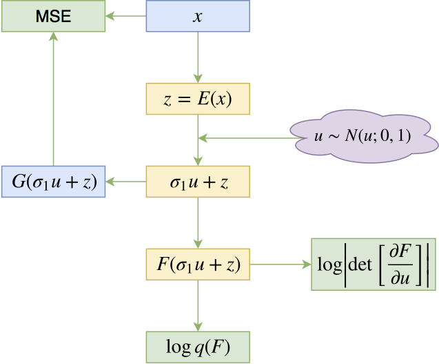
where $\sigma_1,\sigma_2$ are all trainable parameters (scalars suffice), $E(\cdot),G(\cdot)$ are the trainable encoder and decoder (generator), and $F(\cdot)$ is a flow model whose parameters do not depend on $x$. Substituting into $\eqref{eq:f-vae-loss}$, the equivalent loss is
$$\begin{equation}\begin{aligned}\iint \tilde{p}(x)q(u)\bigg[ &\frac{1}{2\sigma_2^2}\Vert G(\sigma_1 u + E(x))-x\Vert^2 + \frac{1}{2}\Vert F(\sigma_1 u + E(x))\Vert^2 \\ &\quad -\log \left|\det \left[\frac{\partial F(\sigma_1 u + E(x))}{\partial u}\right]\right|\bigg] dudx\end{aligned}\end{equation}$$
and the generative sampling process is
$$\begin{equation}u \sim q(u), \quad z = F^{-1}(u),\quad x = G(z)\end{equation}$$
Related work #]
In fact, "flow-based models" is an umbrella term for a large family of models. Besides the coupling-layer-based flows mentioned above (NICE, RealNVP, Glow), there are also "autoregressive flows," represented by works such as PixelRNNs and PixelCNNs. Autoregressive flows usually work well too, but since they generate images pixel by pixel, they can't be parallelized, making generation slow. Flow models like RealNVP and Glow are usually referred to as "normalizing flows," which represent another category of flow model. Glow in particular has made this class of models popular again. In fact, Glow's sampling speed is quite fast — the problem is that its training cycle is too long and training costs are very high.
As far as we know, the first attempt to integrate VAEs with flow models was Variational Inference with Normalizing Flows], followed by two improved works, Improving Variational Inference with Inverse Autoregressive Flow] and Variational Lossy Autoencoder]. Indeed, this line of work (including ours) shares a similar spirit. However, none of the earlier works derived a general framework like our equation $\eqref{eq:f-vae-loss}$, and none of them achieved a major breakthrough in image generation. As far as we can tell, our work is the first to bring RealNVP- and Glow-style coupling-layer flows into VAEs. These "flows" are based on coupling layers $\eqref{eq:coupling}$, which are easy to compute in parallel. So they tend to be more efficient than autoregressive flows and can be stacked very deep. At the same time, we ensure that the latent dimension matches the input dimension; this choice of not reducing dimensionality also helps avoid the blurriness problem.
Experiments #]
Limited by our GPU resources, we only ran experiments at 64x64 and 128x128 resolution on CelebA HQ. We first compare VAEs, Glow, and f-VAEs of similar scale on 64x64 images, then show the generation results at 128x128 in more detail.
Experimental setup #]
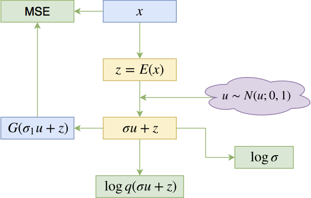
First, our encoder $E(\cdot)$ is a stack of convolutions and Squeeze operators. Specifically, $E(\cdot)$ is composed of several blocks, with a Squeeze operation performed before each block. Each block, in turn, is composed of several steps, each of the form $x + CNN(x)$, where $CNN(x)$ consists of 3x3 and 1x1 convolutions. See the code for further details. As for the decoder (generator) $G(\cdot)$, it is a stack of convolutions and UnSqueeze operators, structurally the inverse of $E(\cdot)$. A $\tanh (\cdot)$ activation can optionally be added at the end of the decoder, though this isn't strictly necessary. The unconditional flow $F(\cdot)$ is taken directly from the Glow model, just not as deep, and with fewer convolutional filters.
Source code (based on Keras 2.2 + TensorFlow 1.8 + Python 2.7):
https://github.com/bojone/flow/blob/master/f-VAEs.py]
 ]
]
Basic structure of VAEs
 ]
]
Basic structure of flow-based models
 ]
]
Basic structure of f-VAEs
Experimental results #]
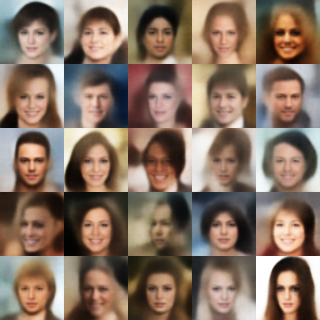
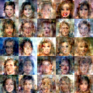
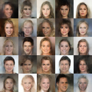
Comparing the results of VAEs and f-VAEs, we can conclude that f-VAEs essentially solve the blurriness problem of VAEs. Comparing Glow and f-VAEs at similar scale, we find that f-VAEs perform better after the same number of epochs. Of course, we don't doubt that Glow could perform just as well, or even better, with a deeper network — but it's clear that at the same complexity and the same training time, f-VAEs perform better.
 ]
]
samples-vae
 ]
]
samples-glow
 ]
]
samples-f-vae
For the 64x64 results, f-VAEs only needed about 120–150 epochs on a GTX 1060, taking roughly 7–8 hours. To be precise, the complete encoder of f-VAEs should be regarded as $F(E(\cdot))$, i.e., the composition of $F$ and $E$. In a standard flow model, we would need to compute the Jacobian determinant of $E$, but in f-VAEs this is not required. So $E$ can just be an ordinary convolutional network, which can supply most of the nonlinearity, thereby reducing the dependence on the flow model $F$.
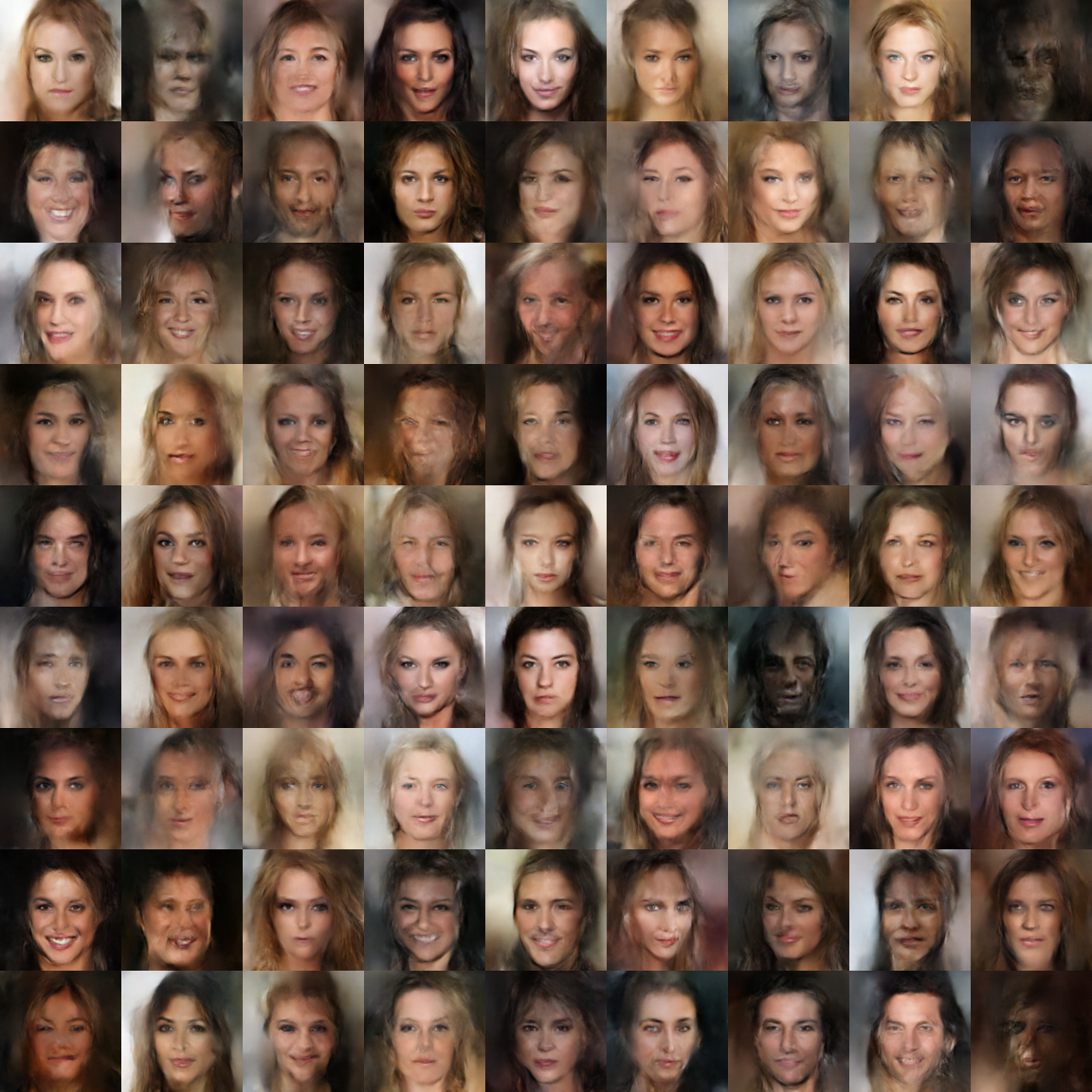
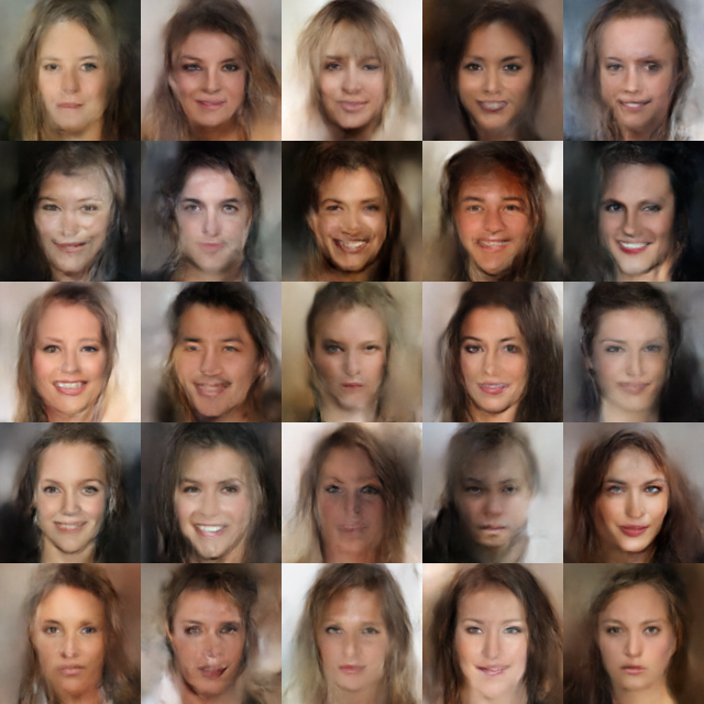
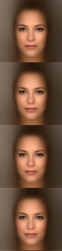
Below are the 128x128 results (the annealing parameter $T$ refers to the standard deviation of the prior distribution). The 128x128 model was trained for about 1.5 days (roughly 150 epochs) on a GTX 1060.
Random samples #]
 ]
]
Samples with annealing parameter 0.8
 ]
]
Samples with annealing parameter 0.8, set 2
Linear interpolation in latent space #]
]
Linear interpolation between two real samples
 ]
]
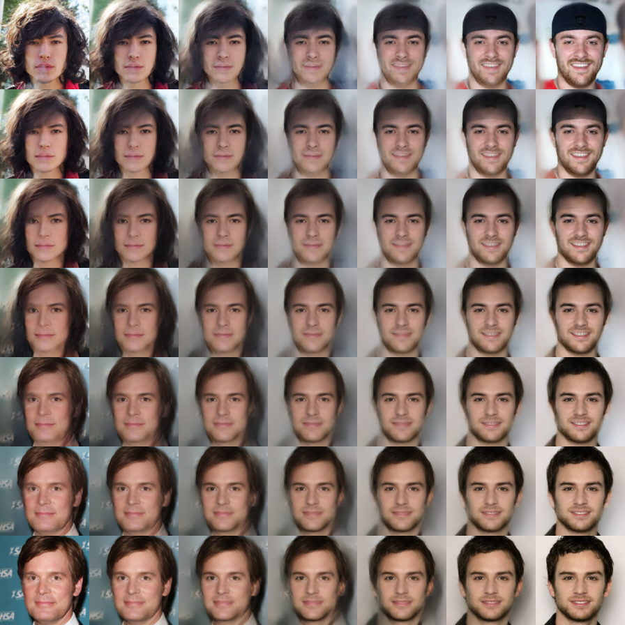
Linear interpolation among four samples, 1
 ]
]
Linear interpolation among four samples, 2
Effect of the annealing parameter #]
 ]
]
T=0.0
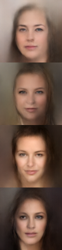 ]
]
T=0.5
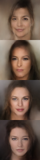 ]
]
T=0.6
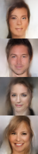 ]
]
T=0.7
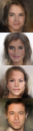 ]
]
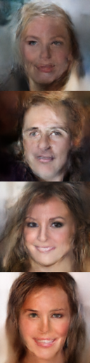
T=0.8
 ]
]
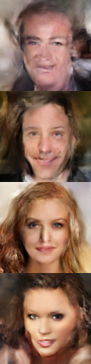
T=0.9
 ]
]
T=1.0
Summary #]
Overview #]
Actually, the original goal of this work was to address two questions raised about Glow: 1) how to reduce Glow's computational cost, and 2) how to obtain a "dimensionality-reducing" version of Glow. Our results show that a non-dimensionality-reducing f-VAE is essentially equivalent to a mini version of Glow, while still achieving good results. And equation $\eqref{eq:f-vae-loss}$ indeed also allows us to train a dimensionality-reducing version of a flow model. We have also proven theoretically that both ordinary VAEs and flow-based models are naturally subsumed within our framework. So our original goal has essentially been accomplished, resulting in a more general framework for generation and inference.
Future work #]
Of course, we can see that the randomly generated images still have a somewhat "oil-painting" feel to them. A possible reason is that the model still isn't complex enough, but we suspect another important factor is the "overuse" of 3x3 convolutions, which leads to an unboundedly expanding receptive field and prevents the model from focusing on fine detail. So, one challenging task ahead is how to design better, more principled encoders and decoders. It seems the ideas from Network in Network] could be valuable here, and the architecture of PGGAN] is also worth trying, though neither has been verified yet.
Translated automatically with claude-sonnet-5; all equations are reproduced verbatim from the source. Copyright remains with the original author.