Variational Autoencoders (IV): A One-Shot Clustering Scheme

变分自编码器（四）：一步到位的聚类方案 苏剑林 · 2018-09-17 · Machine Learning clustering unsupervised VAE generative model

Since VAEs contain both an encoder and a decoder (generator), and since the latent variable distribution is approximately encoded as a standard normal distribution, a VAE is at once a generative model and a feature extractor. In the image domain, since VAE-generated images tend to be blurry, people are usually more interested in the VAE's role as an image feature extractor. Extracted features are always prepared for some downstream task, and there can be many such tasks — classification, clustering, and so on. This post is concerned with the task of "clustering."

Generally speaking, using an AE or VAE for clustering is done in stages: first train an ordinary VAE, obtain the latent variables of the raw data, and then run something like K-Means or a GMM on those latent variables. But this kind of pipeline clearly lacks a sense of unity, and the choice of clustering method is also something we have to agonize over. This post introduces a "one-shot" clustering approach based on VAEs, which allows us to perform unsupervised clustering and conditional generation simultaneously.

Theory

General framework

Let's recall the VAE loss (if it doesn't ring a bell, please refer to Variational Autoencoders (II): From a Bayesian Perspective):

$$KL\Big(p(x,z)\Big\Vert q(x,z)\Big) = \iint p(z|x)\tilde{p}(x)\ln \frac{p(z|x)\tilde{p}(x)}{q(x|z)q(z)} dzdx\tag{1}$$

Usually, we assume that $q(z)$ is a standard normal distribution and $p(z|x),q(x|z)$ is a conditional normal distribution; substituting these in gives us the loss of an ordinary VAE. more

However, nobody ever said the latent variable has to be continuous, right? Here we take the latent variable to be $(z, y)$, where $z$ is a continuous variable representing the encoding vector, and $y$ is a discrete variable representing the category. Directly replacing $z$ in $(1)$ with $(z,y)$ gives us

$$KL\Big(p(x,z,y)\Big\Vert q(x,z,y)\Big) = \sum_y \iint p(z,y|x)\tilde{p}(x)\ln \frac{p(z,y|x)\tilde{p}(x)}{q(x|z,y)q(z,y)} dzdx\tag{2}$$

This is the loss for a VAE used for clustering.

Stage-wise assumptions

What? Is that really it? Well, yes — if we're only considering the general framework, $(2)$ really is all there is to it.

But in practice, $(2)$ can be realized in many different ways; here we introduce a relatively simple one. First, we need to be clear that in $(2)$ we only know $\tilde{p}(x)$ (given as an empirical distribution from a batch of data); everything else is left unspecified. So in order to solve $(2)$, we need to fix some specific forms. One choice is

$$p(z,y|x)=p(y|z)p(z|x),\quad q(x|z,y)=q(x|z),\quad q(z,y)=q(z|y)q(y)\tag{3}$$

Substituting into $(2)$ gives

$$KL\Big(p(x,z,y)\Big\Vert q(x,z,y)\Big) = \sum_y \iint p(y|z)p(z|x)\tilde{p}(x)\ln \frac{p(y|z)p(z|x)\tilde{p}(x)}{q(x|z)q(z|y)q(y)} dzdx\tag{4}$$

Equation $(4)$ is actually quite intuitive — it describes the encoding and generation process:

1. We sample $x$ from the raw data, obtain the encoded feature $z$ via $p(z|x)$, and then classify that encoded feature using the classifier $p(y|z)$ to get its category;
2. We select a category $y$ from the distribution $q(y)$, then draw a random latent variable $z$ from the distribution $q(z|y)$, which is then decoded by the generator $q(x|z)$ back into the original sample.

Concrete model

Equation $(4)$ is already fairly concrete; we just need to follow the usual VAE recipe: $p(z|x)$ is generally assumed to be a normal distribution with mean $\mu(x)$ and variance $\sigma^2(x)$, $q(x|z)$ is generally assumed to be a normal distribution with mean $G(z)$ and constant variance (equivalent to using MSE as the loss), and $q(z|y)$ can be assumed to be a normal distribution with mean $\mu_y$ and variance 1. As for the remaining $q(y),p(y|z)$, $q(y)$ can be assumed to be a uniform distribution (i.e., just a constant), meaning we want each class to be roughly balanced, while $p(y|z)$ is a classifier over the latent variables, which can simply be fit with an ordinary softmax network.

Finally, we can vividly rewrite $(4)$ as

$$\mathbb{E}_{x\sim\tilde{p}(x)}\Big[-\log q(x|z) + \sum_y p(y|z) \log \frac{p(z|x)}{q(z|y)} + KL\big(p(y|z)\big\Vert q(y)\big)\Big],\quad z\sim p(z|x) \tag{5}$$

where $z\sim p(z|x)$ is the reparameterization operation, and the three loss terms in the square brackets each carry their own meaning:

1. $-\log q(x|z)$ wants the reconstruction error to be as small as possible, i.e., it wants $z$ to retain as much complete information as possible;
2. $\sum_y p(y|z) \log \frac{p(z|x)}{q(z|y)}$ wants $z$ to align as closely as possible with some category's "dedicated" normal distribution — this is the step that performs the actual clustering;
3. $KL\big(p(y|z)\big\Vert q(y)\big)$ wants the distribution over classes to be as balanced as possible, so that two classes don't end up nearly coinciding (collapsing into one class). Of course, sometimes this prior requirement isn't needed, in which case this term can simply be dropped.

Experiments

The experimental code was naturally done in Keras (^_^), and experiments were run on MNIST and Fashion-MNIST, both with decent performance. Experimental environment: Keras 2.2 + TensorFlow 1.8 + Python 2.7.

Code implementation

The code is located at: https://github.com/bojone/vae/blob/master/vae_keras_cluster.py

The comments should be fairly clear, and the changes compared to an ordinary VAE aren't large. The one part that might be slightly tricky is how to implement $\sum_y p(y|z) \log \frac{p(z|x)}{q(z|y)}$. First we substitute in

$$\begin{aligned}p(z|x)&=\frac{1}{\prod\limits_{i=1}^d\sqrt{2\pi\sigma_i^2(x)}}\exp\left\{-\frac{1}{2}\left\Vert\frac{z - \mu(x)}{\sigma(x)}\right\Vert^2\right\}\\ q(z|y)&=\frac{1}{(2\pi)^{d/2}}\exp\left\{-\frac{1}{2}\left\Vert z - \mu_y\right\Vert^2\right\}\end{aligned}\tag{6}$$

to get

$$\log \frac{p(z|x)}{q(z|y)}=-\frac{1}{2}\sum_{i=1}^d \log \sigma_i^2(x)-\frac{1}{2}\left\Vert\frac{z - \mu(x)}{\sigma(x)}\right\Vert^2 + \frac{1}{2}\left\Vert z - \mu_y\right\Vert^2 \tag{7}$$

Note that the second term is actually redundant, because the reparameterization operation tells us that $z = \varepsilon\otimes \sigma(x) + \mu(x),\,\varepsilon\sim \mathcal{N}(0,1)$, so the second term is in fact just $-\Vert \varepsilon\Vert^2/2$, which is independent of the parameters. So $$\log \frac{p(z|x)}{q(z|y)}\sim -\frac{1}{2}\sum_{i=1}^d \log \sigma_i^2(x) + \frac{1}{2}\left\Vert z - \mu_y\right\Vert^2 \tag{8}$$

Then, since $y$ is discrete, $\sum_y p(y|z) \log \frac{p(z|x)}{q(z|y)}$ is in fact just a matrix multiplication (multiplying and then summing over some shared variable is exactly the general form of matrix multiplication), which is implemented using K.batch_dot.

Beyond that, readers should already be familiar with how ordinary VAEs are implemented before diving into this post and its code — otherwise it's probably going to be a bit bewildering.

MNIST

Here are the MNIST experimental results, showing both within-class samples and per-class sampling. Finally, I did a rough estimate: if we assign each cluster the label of whichever true class is most represented in it, the resulting test accuracy is about 83%. Compared with the results in Unsupervised Deep Embedding for Clustering Analysis (whose best result is also around 84%), this seems pretty solid.

Clustering illustration

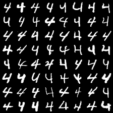Cluster category_0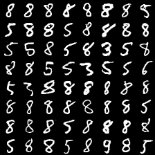Cluster category_1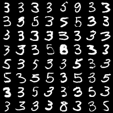Cluster category_2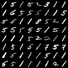Cluster category_3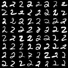Cluster category_4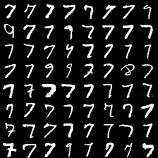Cluster category_5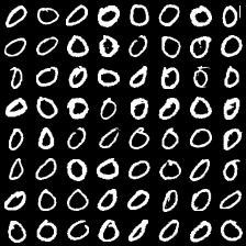Cluster category_6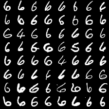Cluster category_7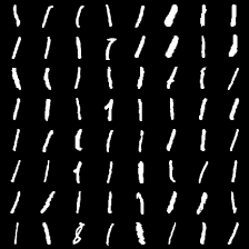Cluster category_8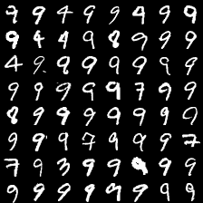Cluster category_9

Per-class sampling

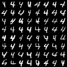Class sample_0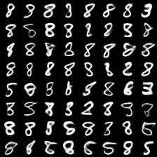Class sample_1Class sample_2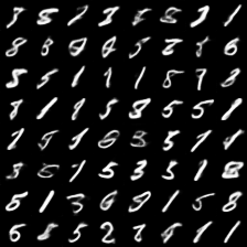Class sample_3Class sample_4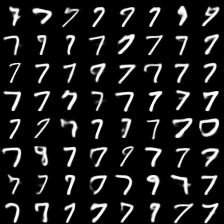Class sample_5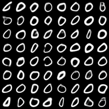Class sample_6Class sample_7Class sample_8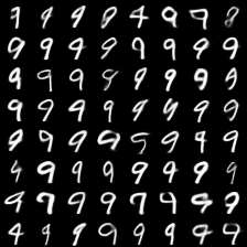Class sample_9

Fashion-MNIST

Here are the experimental results on Fashion-MNIST, showing both within-class samples and per-class sampling; the final test accuracy is about 58.5%.

Clustering illustration

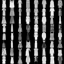Cluster category_0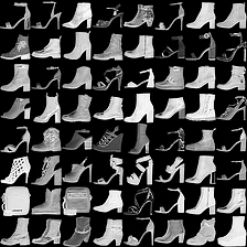Cluster category_1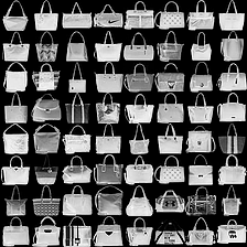Cluster category_2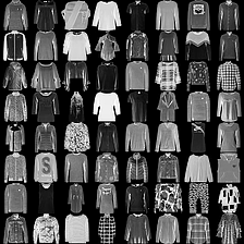Cluster category_3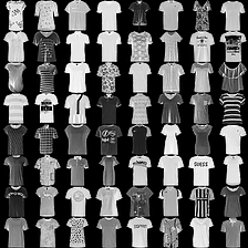Cluster category_4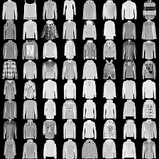Cluster category_5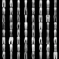Cluster category_6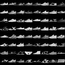Cluster category_7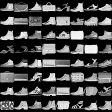Cluster category_8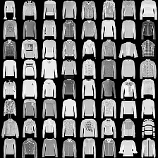Cluster category_9

Per-class sampling

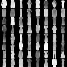Class sample_0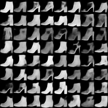Class sample_1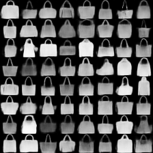Class sample_2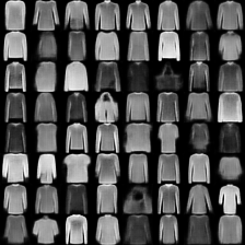Class sample_3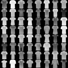Class sample_4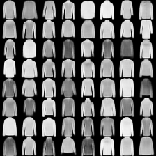Class sample_5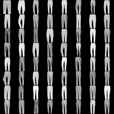Class sample_6Class sample_7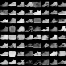Class sample_8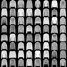Class sample_9

Summary

This post implements a simple VAE-based clustering algorithm in a straightforward manner. The distinctive feature of the algorithm is that it's done in one shot, accomplishing "encoding," "clustering," and "generation" all together, with the underlying idea being a generalization of the VAE loss.

There's likely still room for improvement — for instance, equation $(4)$ is just one example of the more general form in equation $(2)$, and more general cases could still be considered. Neither the encoder nor the decoder in the code has been carefully tuned; they're only there to verify the idea.