A Conv1D-Based Spectral Classification Model (1D Sequence Classification)

基于Conv1D的光谱分类模型（一维序列分类） 苏剑林 · 2018-05-02 · Machine Learning model astronomy spectrum

A while back Tianchi launched an astronomical data-mining competition — LAMOST Spectral Classification (identifying the corresponding spectrum as one of 4 classes). Even though there was no prize money, it looked interesting, so I signed up. After working on it for a while, I felt my results were decent, but in the end I forgot (or rather, never even noticed) that in the last two days of the preliminary round there was a step to submit results on a new test set — and that was that. It left behind an unfinished model, a case of "dying before achieving victory," except this time I killed it myself.

Astronomical Data Mining Competition — Intelligent Classification of Celestial Spectra

Later, after discussing this with other participants, I realized my model was actually pretty good. As I recall, the first-place score in the preliminary round was 0.83+, while mine was 0.82+, ranking around 4th or 5th. Apparently many of the teams scoring 0.8+ had already used ensemble models, whereas my 0.82+ score was from a single model alone. I've also noticed in group chats that quite a few friends are working on 1D sequence classification models, and spectral classification is essentially just 1D sequence classification at its core. So I figured I'd share the model — it should be of some reference value to people working on related problems.

The Model

Honestly it's nothing special — just ordinary 1D convolutions with residual connections. For anyone familiar with image processing, this is about as ordinary a structure as it gets. more

CNN model for spectral recognitionBlock structure diagram of the spectral CNN

The form of each Conv1D block is shown in the diagram on the right; see the code below for the specific parameters.

Rationale

Let me also say a word about why CNNs work well here.

Features suitable for CNNs should satisfy local correlation, meaning that the relationships between features are mainly expressed locally, and extend from the local to the global. Clearly, both images and audio satisfy this property, which is why mainstream image and audio recognition models today rely on CNNs.

As for spectral sequences, they're essentially like a function graph (2600 points), as shown below. They also exhibit local correlation, so we use CNNs to tackle the problem. Of course, using an RNN model such as LSTM isn't impossible either, but RNNs can't be parallelized, which is intolerable for such long sequences. To use 1D convolutions, we need to convert the sequence into the $2600\times 1$ format. Additionally, we know that the human eye identifies spectra by recognizing emission and absorption lines — in simple terms, these are features with relatively large differences. To capture such features, we use max pooling for all pooling layers, and use only the ReLU activation function [since relu(x)=max(x,0)].

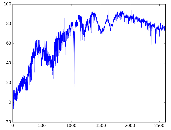Reference spectrum example

Additionally, since these sequences are quite long (up to 2600 dimensions), a few tricks were used: dilated convolutions, along with as many blocks as possible, each followed by a pooling layer for dimensionality reduction.

Training

Before giving the training code, let me first describe the training process.

The competition's evaluation metric is the macro F1 score, meaning an F1 score is computed for each class, and then the four classes' F1 values are averaged. Generally speaking, F1 values are not differentiable, so the macro F1 score is also not differentiable and cannot be directly used as a loss. However, we can write an approximate formula for (the negative of) the macro F1 score:

def score_loss(y_true, y_pred):
    loss = 0
    for i in np.eye(4):
        y_true_ = K.constant([list(i)]) * y_true
        y_pred_ = K.constant([list(i)]) * y_pred
        loss += 0.5 * K.sum(y_true_ * y_pred_) / K.sum(y_true_ + y_pred_ + K.epsilon())
    return - K.log(loss + K.epsilon())

where y_true is the one-hot distribution of the target, and y_pred is the predicted probability for each class. This may seem hard to understand at first glance — readers need to understand how F1 is computed, and then express that computation in a form suitable for one-hot inputs, in order to gradually make sense of it.

To optimize for this evaluation metric, I first trained the model to optimality using the Adam optimizer (learning rate 0.001) with ordinary categorical cross-entropy, and then switched to the score_loss, lowering the learning rate to 0.0001, and continued training the model to optimality. This process is reflected in the code. Interestingly, training directly with the macro F1 score as the loss fails to converge at all — a somewhat curious phenomenon.

Code

Below is the reference code, which indeed has nothing particularly special about it. If you have any questions, feel free to leave a comment for discussion.

#! -*- coding: utf-8 -*-

import numpy as np
import os,glob
import pandas as pd
import json
import keras.backend as K
from keras.callbacks import Callback
from keras.utils import to_categorical
from tqdm import tqdm
np.random.seed(2018)

# 数据读取。
# 光谱的存储方式为一个txt存一个样本，txt里边是字符串格式的序列
# 对于做其他序列分类的读者，只需要知道这里就是生成序列的样本就就行了
class Data_Reader:
    def __init__(self):
        self.labels = pd.read_csv('../first_train_index_20180131.csv')
        self.label2id = {'star':0, 'unknown':1, 'galaxy':2, 'qso':3}
        self.id2label = ['star', 'unknown', 'galaxy', 'qso']
        self.labels['type'] = self.labels['type'].apply(lambda s: self.label2id[s])
        self.labels = dict(zip(self.labels['id'], self.labels['type']))
        if os.path.exists('../train_data.json'): # 读取保存好的数据
            print 'Found. Reading ...'
            self.train_data = json.load(open('../train_data.json'))
            self.valid_data = json.load(open('../valid_data.json'))
            self.nb_train = len(self.train_data)
            self.nb_valid = len(self.valid_data)
        else: # 如果还没有保存好，则直接从原始数据构建
            print 'Not Found. Preparing ...'
            self.data = glob.glob('../train/*.txt')
            np.random.shuffle(self.data)
            self.train_frac = 0.8
            self.nb_train = int(self.train_frac*len(self.data))
            self.nb_valid = len(self.data) - self.nb_train
            self.train_data = self.data[:self.nb_train]
            self.valid_data = self.data[self.nb_train:]
            json.dump(self.train_data, open('../train_data.json', 'w'))
            json.dump(self.valid_data, open('../valid_data.json', 'w'))
        self.input_dim = len(self.read_one(self.train_data[0]))
        self.fracs = [0.8, 0.1, 0.05, 0.05] # 每个batch中，每一类的采样比例
        self.batch_size = 160 # batch_size
        for i in range(4):
            self.fracs[i] = int(self.fracs[i]*self.batch_size)
        self.fracs[0] = self.batch_size - np.sum(self.fracs[1:])
    def read_one(self, fn):
        return np.array(json.loads('[' + open(fn).read() + ']'))
    def for_train(self): # 生成训练集
        train_data = [[], [], [], []]
        for n in self.train_data:
            train_data[self.labels[int(n.split('/')[2].split('.')[0])]].append(n)
        print 'Samples:',self.fracs
        Y = np.array([0]*self.fracs[0] + [1]*self.fracs[1] + [2]*self.fracs[2] + [3]*self.fracs[3])
        Y = to_categorical(np.array(Y), 4)
        while True:
            X = []
            for i in range(4):
                for n in np.random.choice(train_data[i], self.fracs[i]):
                    X.append(self.read_one(n))
            X = np.expand_dims(np.array(X), 2)/100.
            yield X,Y
            X = []
    def for_valid(self): # 生成验证集
        X,Y = [],[]
        for n in self.valid_data:
            X.append(self.read_one(n))
            Y.append(self.labels[int(n.split('/')[2].split('.')[0])])
            if len(X) == self.batch_size or n == self.valid_data[-1]:
                X = np.expand_dims(np.array(X), 2)/100.
                Y = to_categorical(np.array(Y), 4)
                yield X,Y
                X,Y = [],[]

D = Data_Reader()

from keras.layers import *
from keras.models import Model
import keras.backend as K

def BLOCK(seq, filters): # 定义网络的Block
    cnn = Conv1D(filters*2, 3, padding='SAME', dilation_rate=1, activation='relu')(seq)
    cnn = Lambda(lambda x: x[:,:,:filters] + x[:,:,filters:])(cnn)
    cnn = Conv1D(filters*2, 3, padding='SAME', dilation_rate=2, activation='relu')(cnn)
    cnn = Lambda(lambda x: x[:,:,:filters] + x[:,:,filters:])(cnn)
    cnn = Conv1D(filters*2, 3, padding='SAME', dilation_rate=4, activation='relu')(cnn)
    cnn = Lambda(lambda x: x[:,:,:filters] + x[:,:,filters:])(cnn)
    if int(seq.shape[-1]) != filters:
        seq = Conv1D(filters, 1, padding='SAME')(seq)
    seq = add([seq, cnn])
    return seq

#搭建模型，就是常规的CNN加残差加池化
input_tensor = Input(shape=(D.input_dim, 1))
seq = input_tensor

seq = BLOCK(seq, 16)
seq = MaxPooling1D(2)(seq)
seq = BLOCK(seq, 16)
seq = MaxPooling1D(2)(seq)
seq = BLOCK(seq, 32)
seq = MaxPooling1D(2)(seq)
seq = BLOCK(seq, 32)
seq = MaxPooling1D(2)(seq)
seq = BLOCK(seq, 64)
seq = MaxPooling1D(2)(seq)
seq = BLOCK(seq, 64)
seq = MaxPooling1D(2)(seq)
seq = BLOCK(seq, 128)
seq = MaxPooling1D(2)(seq)
seq = BLOCK(seq, 128)
seq = Dropout(0.5, (D.batch_size, int(seq.shape[1]), 1))(seq)
seq = GlobalMaxPooling1D()(seq)
seq = Dense(128, activation='relu')(seq)

output_tensor = Dense(4, activation='softmax')(seq)

model = Model(inputs=[input_tensor], outputs=[output_tensor])
model.summary()

# 定义marco f1 score的相反数作为loss
def score_loss(y_true, y_pred):
    loss = 0
    for i in np.eye(4):
        y_true_ = K.constant([list(i)]) * y_true
        y_pred_ = K.constant([list(i)]) * y_pred
        loss += 0.5 * K.sum(y_true_ * y_pred_) / K.sum(y_true_ + y_pred_ + K.epsilon())
    return - K.log(loss + K.epsilon())

# 定义marco f1 score的计算公式
def score_metric(y_true, y_pred):
    y_true = K.argmax(y_true)
    y_pred = K.argmax(y_pred)
    score = 0.
    for i in range(4):
        y_true_ = K.cast(K.equal(y_true, i), 'float32')
        y_pred_ = K.cast(K.equal(y_pred, i), 'float32')
        score += 0.5 * K.sum(y_true_ * y_pred_) / K.sum(y_true_ + y_pred_ + K.epsilon())
    return score

from keras.optimizers import Adam
model.compile(loss='categorical_crossentropy', # 交叉熵作为loss
              optimizer=Adam(1e-3),
              metrics=[score_metric])

try:
    model.load_weights('guangpu_highest.model')
except:
    pass

def predict():
    import time
    data = pd.read_csv('../first_test_index_20180131.csv')['id']
    data = '../test/' + data.apply(str) + '.txt'
    data = list(data)
    I,X,Y = [],[],[]
    for n in tqdm(iter(data)):
        X.append(D.read_one(n))
        I.append(int(n.split('/')[2].split('.')[0]))
        if len(X) == D.batch_size:
            X = np.expand_dims(np.array(X), 2)/100.
            y = model.predict(X)
            y = y.argmax(axis=1)
            Y.extend(list(y))
            X = []
    d = pd.DataFrame(list(zip(I, Y)))
    d.columns = ['id', 'type']
    d['type'] = d['type'].apply(lambda s: D.id2label[s])
    d.to_csv('result_%s.csv'%(int(time.time())), index=None, header=None)

if __name__ == '__main__':
    
    # 定义Callback器，计算验证集的score，并保存最优模型
    class Evaluate(Callback):
        def __init__(self):
            self.scores = []
            self.highest = 0.
        def on_epoch_end(self, epoch, logs=None):
            R,T = [],[]
            for x,y in D.for_valid():
                y_ = model.predict(x)
                R.extend(list(y.argmax(axis=1)))
                T.extend(list(y_.argmax(axis=1)))
            R,T = np.array(R),np.array(T)
            score = 0
            for i in range(4):
                R_ = (R == i)
                T_ = (T == i)
                score += 0.5 * (R_ * T_).sum() / (R_.sum() + T_.sum() + K.epsilon())
            self.scores.append(score)
            if score >= self.highest: # 保存最优模型权重
                self.highest = score
                model.save_weights('guangpu_highest.model')
            json.dump([self.scores, self.highest], open('valid.log', 'w'))
            print '            score: %f%%, highest: %f%%'%(score*100, self.highest*100)

    evaluator = Evaluate()

    # 第一阶段训练
    history = model.fit_generator(D.for_train(),
                                  steps_per_epoch=500,
                                  epochs=50,
                                  callbacks=[evaluator])

    model.compile(loss=score_loss, # 换一个loss
                  optimizer=Adam(1e-4),
                  metrics=[score_metric])

    try:
        model.load_weights('guangpu_highest.model')
    except:
        pass

    # 第二阶段训练
    history = model.fit_generator(D.for_train(),
                                  steps_per_epoch=500,
                                  epochs=50,
                                  callbacks=[evaluator])