*Equations and the Universe*: The Comings and Goings of the Two-Body Problem (Part 1)
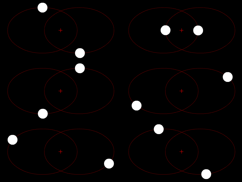 Orbital simulation of the two-body problem
To make content on "celestial mechanics" more accessible, and at the same time to sharpen my own skills in exposition and computation, I (BoJone) came up with the idea for a series called Equations and the Universe, whose main purpose is to discuss some astronomical problems using mathematics in reasonably serious depth. I've always felt that it's impossible to describe science perfectly without using formulas (though of course one shouldn't rely on formulas alone either). I remember that Hawking's A Brief History of Time and The Universe in a Nutshell, among other books, went to great lengths to use no math—or as little as possible—to express his ideas. This approach works well for a general audience, but it's not very helpful for readers who want to dig deeper. So my position is: the universe is something you compute!
Every word of this series is typed by BoJone himself, drawing in places on material from Introduction to Celestial Mechanics, along with some of my own personal insights. Because of the length involved and limited time, I plan to publish this in several installments, and I'll try to keep the language as accessible as possible, so that anyone with a bit of calculus background can follow along. Here I'm posting the first installment. Given the time constraints, there may well be some oversights—corrections are very welcome! more
The two-body problem asks how two celestial bodies move under mutual gravitational attraction (classical Newtonian mechanics), assuming no interference from any other bodies. This is the simplest class of problem in celestial mechanics, and currently the only type that can be solved exactly. Once you bring in three or more bodies, you're limited to approximate analysis or numerical methods.
Suppose we have only the Sun S and a single planet P. Set up an arbitrary spatial coordinate system O-xyz, where $\boldsymbol{r}_s$ is the position vector of the Sun and $\boldsymbol{r}_p$ is the position vector of the planet. $\boldsymbol{r}$ is then the position vector of the planet relative to the Sun. Let M and m denote the masses of the Sun and the planet, respectively. The gravitational force exerted on the Sun by the planet is
$$\boldsymbol{F}_s=G\frac{Mm}{r^2}\frac{\boldsymbol{r}}{|\boldsymbol{r}|}=G\frac{Mm}{r^3}\boldsymbol{r}$$
while the gravitational force exerted on the planet by the Sun is
$$\boldsymbol{F}_p=G\frac{Mm}{r^2}\frac{-\boldsymbol{r}}{|\boldsymbol{r}|}=-G\frac{Mm}{r^3}\boldsymbol{r}$$
By Newton's second law, both the Sun and the planet undergo motion driven by these forces:
$$\boldsymbol{F}=\frac{d(mv)}{dt}=m\frac{d^2 \boldsymbol{r}}{dt^2}$$
so we must have
$$\begin{aligned}\boldsymbol{F}_s=G\frac{Mm}{r^3}\boldsymbol{r}=M\frac{d^2 \boldsymbol{r}_s}{dt^2} \\ \boldsymbol{F}_p=-G\frac{Mm}{r^3}\boldsymbol{r}=m\frac{d^2 \boldsymbol{r}_p}{dt^2}\end{aligned}$$
Since $\boldsymbol{r}=\boldsymbol{r}_p-\boldsymbol{r}_s$, this gives
$$\frac{d^2 \boldsymbol{r}}{dt^2}=\frac{d^2}{dt^2}(\boldsymbol{r}_p-\boldsymbol{r}_s)=-\frac{\mu}{r^3}\boldsymbol{r}$$
where $\mu=G(M+m)$. If we set up a Cartesian x-y-z coordinate system with the Sun at the origin, we obtain the system of differential equations for the two-body problem:
$$\begin{aligned}\frac{d^2 x}{dt^2}=-\frac{\mu}{r^3}x \\ \frac{d^2 y}{dt^2}=-\frac{\mu}{r^3}y \\ \frac{d^2 z}{dt^2}=-\frac{\mu}{r^3}z\end{aligned}$$
where $r^2=x^2+y^2+z^2$. Let's now look at how to solve this system of equations. From theoretical mechanics we know that the planet's motion is governed by a central force, and motion under a central force is always planar—though of course we can also verify this directly from the differential equations above. From the last two equations of the system we get:
$$y\ddot z-z\ddot y=0\Rightarrow \frac{d}{dt}(y\dot z-z\dot y)=0$$
Integrating both sides:
$$y\dot z-z\dot y=A\tag{1}$$
where A is a constant of integration. By the same reasoning we can obtain:
$$z\dot x-x\dot z=B\tag{2}$$$$x\dot y-y\dot x=C\tag{3}$$
Equations (1), (2), (3) are called the "integrals of angular momentum."
Multiplying (1), (2), (3) by x, y, z respectively and adding them together gives:
$Ax+By+Cz=0$
This is the equation of a plane passing through the origin (the Sun), which shows that the planet and the Sun always lie in the same plane! So we only need to consider the equations restricted to the O-xy plane, i.e.
$\ddot x=-\frac{\mu x}{r^3}$, $$\ddot y=-\frac{\mu y}{r^3}\tag{4}$$
the integral of angular momentum then reduces to a single equation: $$x\dot y-y\dot x=h\tag{5}$$
Let's now work in polar coordinates: set $x=rcos\theta,y=rsin\theta$, and (4) becomes
$$\ddot{r} -r\dot{\theta}^2=-\frac{\mu}{r^2}\tag{6}$$
(5) becomes:
$$r^2 \dot{\theta}=h\tag{7}$$
Equation (7) is called the "area integral": h is twice the areal velocity swept out by the radius vector. Since the areal velocity is constant, equal areas are swept out in equal times—and with that we've proven "Kepler's Second Law."
Appendix: a brief sketch of the derivation:
Let $x=r*cos\theta,y=r*sin\theta$........(00)
We have $x^2+y^2=r^2$. Substituting into the original equation
$\ddot{x}=-\frac{\mu cos\theta}{r^2}$, $\ddot{y}=-\frac{\mu sin\theta}{r^2}$........(0)
Differentiating (00) with respect to t:
$\dot{x}=\dot{r}*cos\theta-\dot{\theta}*r*sin\theta$..........(01)
$\dot{y}=\dot{r}*sin\theta+\dot{\theta}*r*cos\theta$..........(02)
Differentiating (01) and (02) again with respect to t:
$\ddot{x}=\ddot{r}*cos\theta-2*\dot{r}*\dot{\theta}*sin\theta-\ddot{\theta}*r*sin\theta-\dot{\theta}^2*r*cos\theta$.....................(03)
$\ddot{y}=\ddot{r}*sin\theta+2*\dot{r}*\dot{\theta}*cos\theta+\ddot{\theta}*r*cos\theta-\dot{\theta}^2*r*sin\theta.$....................(04)
From $(03)*cos\theta+(04)*sin\theta$ we get
$\ddot{x}cos\theta+\ddot{y}sin\theta=\ddot{r}-\dot{\theta}^2*r$.....(05)
And from (0) we also have
$\ddot{x}cos\theta+\ddot{y}sin\theta=-{\mu}/r^2$.......(06)
Comparing (05) and (06) gives
$$\ddot{r}-\dot{\theta}^2\cdot r=-{\mu}/r^2$$
As for going from (5) to (7), that doesn't require any special tricks—just substitute directly, differentiate, and simplify.
Now let's solve the system of equations formed by (6) and (7). If we want to find the curve type of the planet's orbit, we need to find the relationship between r and $\theta$; if we want to compute the planet's position at a given time, we need to find r or $\theta$ as a function of time t.
Let's first work out the type of curve traced by the orbit. Here I'll quote directly from Introduction to Celestial Mechanics.
Let $u=1/r$, then (7) becomes: $\dot{\theta}=hu^2$, and we also have
$$\begin{aligned}\dot{r}=\frac{dr}{d\theta}\frac{d\theta}{dt}=\frac{d(1/u)}{d\theta}\dot{\theta}=-1/u^2\cdot \frac{du}{d\theta}\cdot hu^2=-h\frac{du}{d\theta} \\ \ddot{r}=-h\frac{d}{d\theta}(\frac{du}{d\theta})\dot{\theta}=-h^2 u^2\frac{d^2 u}{d\theta^2}\end{aligned}$$
Substituting this into (6) gives
$$\frac{d^2 u}{d\theta^2}+u=\frac{\mu}{h^2}$$
This is a second-order linear differential equation. Its general solution is:
$$u=\frac{\mu}{h^2}[1+e \cos(\theta-\omega)]\tag{8}$$
where e and $\omega$ are constants to be determined. Converting back to r, this becomes:
$$r=\frac{h^2//\mu}{1+e \cos(\theta-\omega)}\tag{9}$$
From analytic geometry we know this is a conic section with its focus at the origin (an ellipse, hyperbola, or parabola—see Wikipedia for reference). With this we've proven "Kepler's First Law," and in fact in a more general form (not just ellipses, but also hyperbolas and parabolas). From this we can derive $h^2=\mu a(1-e^2)$, where a is the semi-major axis of the conic section, and e is the eccentricity; and when $\theta=\omega$, r attains its minimum value, i.e., the planet is at perihelion, so $\omega$ is the argument of perihelion.
Appendix: how do we solve this differential equation?
For the details of solving this linear differential equation, see Wikipedia.
Using the standard method, we can find that the general solution of $\frac{d^2 u}{d\theta^2}+u=0$ is $y=C_1 cos\theta+C_2 sin\theta$; adding the particular solution $\frac{\mu}{h^2}$ on the right-hand side gives the general solution of the differential equation. But how do we convert this into the form of (8)?
It's not hard to see that $C_1 cos\theta+C_2 sin\theta+\frac{\mu}{h^2}$ is in fact equivalent to (8), because
$$e \cos(\theta-\omega)=ecos\theta \cos\omega+e \sin\theta \sin\omega$$
that is, $ecos\omega=C_1 h^2/{\mu},esin\omega=C_2 h^2/{\mu}$
At this point we've done most of the work; there's just one more small piece left, and then the two-body problem will be completely solved: we need to find r or $\theta$ as a function of time t, so that we can compute the planet's position at any given moment.
Appendix: the relationship between t and r
From (7) we get $\dot{\theta}=h/r^2$. Substituting into (6) gives:
$$\ddot{r} -h^2/r^3=-\frac{\mu}{r^2}\tag{10}$$
This is a second-order differential equation, and its solution isn't hard to find in principle, but the resulting integral is quite messy:
$$\dot{r}\frac{d\dot{r}}{dr}=h^2/r^3-\frac{\mu}{r^2}$$
$\dot{r}d\dot{r}=(h^2/r^3-\frac{\mu}{r^2})dr$, integrating both sides
$$\dot{r}^2={2\mu}/r-h^2/r^2+K_1\tag{11}$$$$\begin{aligned}\Rightarrow {dt}/{dr}=\frac{r}{\sqrt{K_1 r^2+2\mu r-h^2}} \\ t=\int \frac{r}{\sqrt{K_1 r^2+2\mu r-h^2}}dr\end{aligned}$$
This integral is easy enough to evaluate (see this site's
table of integrals
), but the drawback is that the final result comes out in a rather unwieldy form!
What Introduction to Celestial Mechanics actually derives is the relationship between $\theta$ and t (i.e., Kepler's equation)... (to be continued)
Translated automatically with claude-sonnet-5; all equations are reproduced verbatim from the source. Copyright remains with the original author.