Variational Autoencoders (III): Why Does This Approach Actually Work?
I've noticed that I've been fond of writing long-winded articles lately, and they tend to come in clusters — I just wrote three consecutive pieces introducing Capsules, and now it's VAE's turn again. This is the third installment of exploring VAE, and there may well be a fourth. Either way, quantity doesn't matter; what matters is thinking the problem through clearly. This is especially true for a novel modeling paradigm like VAE, which is worth scrutinizing carefully.
The question we care about this time is: why does VAE actually work?
I imagine readers who study VAE go through a few stages. The first stage is right after reading the VAE introduction, feeling completely lost — it seems like an autoencoder but also not quite, and only after gnawing through the text several times and looking at the source code do you get a rough sense of what's going on. The second stage builds on the first: you dig deeper into VAE's principles — latent variable models, KL divergence, variational inference, and so on. Going through it carefully, you find that despite all the twists and turns, you can eventually make sense of everything.
At this point, readers may enter a third stage. In this stage, we start having many doubts, especially about feasibility: "Why does this convoluted process end up producing a workable model? I also have lots of ideas — why don't my ideas work?"
The Essentials So Far
Let's once again patiently review some of the principles of VAE covered previously.
VAE aims to describe the distribution of data $X$ through a latent-variable decomposition
$$p(x)=\int p(x|z)p(z)dz,\quad p(x,z) = p(x|z)p(z)\tag{1}$$
Then $p(x|z)$ is fit with model $q(x|z)$, and $p(z)$ is fit with model $q(z)$. To give the model generative capability, $q(z)$ is defined as a standard normal distribution.
In theory, we could solve for the model by maximizing the marginal likelihood:
$$\begin{aligned}q(x|z)=&\mathop{\text{argmax}}_{q(x|z)} \int \tilde{p}(x)\ln\left(\int q(x|z)q(z)dz\right)dx\\ =&\mathop{\text{argmax}}_{q(x|z)} \mathbb{E}_{x\sim\tilde{p}(x)}\left[\ln\left(\int q(x|z)q(z)dz\right)\right] \end{aligned}\tag{2}$$
But since the integral inside the parentheses can't be computed explicitly, we instead introduce KL divergence to measure the discrepancy between joint distributions, and the final objective becomes
$$\begin{aligned}\mathcal{L} =&\mathbb{E}_{x\sim \tilde{p}(x)} \left[-\int p(z|x)\ln q(x|z)dz+\int p(z|x)\ln \frac{p(z|x)}{q(z)}dz\right]\\ = &\mathbb{E}_{x\sim \tilde{p}(x)} \left[\mathbb{E}_{z\sim p(z|x)}\big[-\ln q(x|z)\big]+\mathbb{E}_{z\sim p(z|x)}\Big[\ln \frac{p(z|x)}{q(z)}\Big]\right]\end{aligned}\tag{3}$$
By minimizing $\mathcal{L}$, we solve for $p(z|x)$ and $q(x|z)$ separately. The previous post, Variational Autoencoders (II): From a Bayesian Perspective], also showed that $\mathcal{L}$ has a lower bound $-\mathbb{E}_{x\sim \tilde{p}(x)}\big[\ln \tilde{p}(x)\big]$, so comparing how close $\mathcal{L}$ is to $-\mathbb{E}_{x\sim \tilde{p}(x)}\big[\ln \tilde{p}(x)\big]$ lets us gauge the relative quality of the generator.
The Puzzle of Sampling
In this section, we try to interrogate VAE's principles closely, hoping to answer why VAE does what it does, and — most crucially — why doing so actually works.
Sampling a Single Point Is Enough
For equation $(3)$, we previously handled it as follows:
1. Notice that $\mathbb{E}_{z\sim p(z|x)}\Big[\ln \frac{p(z|x)}{q(z)}\Big]$ is exactly the divergence $KL\Big(p(z|x)\Big\Vert q(z)\Big)$ between $p(z|x)$ and $q(z)$, and since we've assumed both are normal distributions, this term can be computed in closed form;
2. For the term $\mathbb{E}_{z\sim p(z|x)}\big[-\ln q(x|z)\big]$, we assume that sampling a single point is representative enough, so this term becomes $-\ln q(x|z),\, z\sim p(z|x)$.
After this treatment, the whole loss can be written explicitly:
$$\mathcal{L}=\mathbb{E}_{x\sim \tilde{p}(x)} \left[-\ln q(x|z) + KL\Big(p(z|x)\Big\Vert q(z)\Big)\right],\quad z\sim p(z|x)\tag{4}$$
Wait — some readers might object: $KL\Big(p(z|x)\Big\Vert q(z)\Big)$ is computed exactly beforehand, which is equivalent to sampling infinitely many points to estimate that term; yet $\mathbb{E}_{z\sim p(z|x)}\big[-\ln q(x|z)\big]$ only samples a single point. Both are part of the loss — is this unequal treatment really fair?
In fact, $\mathbb{E}_{z\sim p(z|x)}\Big[\ln \frac{p(z|x)}{q(z)}\Big]$ can also be computed by sampling just a single point. That is, by having everything use only a single sample, we can turn equation $(3)$ into
$$\begin{aligned}\mathcal{L} =&\mathbb{E}_{x\sim \tilde{p}(x)} \left[-\ln q(x|z)+\ln \frac{p(z|x)}{q(z)}\right]\\ =&\mathbb{E}_{x\sim \tilde{p}(x)} \Big[-\ln q(x|z)+\ln p(z|x) - \ln q(z)\Big]\,,\quad z\sim p(z|x) \end{aligned}\tag{5}$$
Although this loss differs somewhat from the standard VAE, it in fact converges to a similar result.
Why Is One Sample Enough?
So why is sampling a single point sufficient? Under what conditions is one sample enough?
First, let me give an example of "one sample is not enough." Let's revisit equation $(2)$, which can actually be rewritten as:
$$q(x|z)=\mathop{\text{argmax}}_{q(x|z)} \mathbb{E}_{x\sim\tilde{p}(x)}\Bigg[\ln\Big(\mathbb{E}_{z\sim q(z)}\big[q(x|z)\big]\Big)\Bigg]\tag{6}$$
If sampling one point were enough — no, let's be cautious and say we sample $k$ points — then we could write
$$q(x|z)=\mathop{\text{argmax}}_{q(x|z)} \mathbb{E}_{x\sim\tilde{p}(x)}\Bigg[\ln\left(\frac{1}{k}\sum_{i=1}^k q(x|z_i)\right)\Bigg],\quad z_1,\dots,z_k \sim q(z)\tag{7}$$
and then train by gradient descent.
However, this strategy does not succeed. In practice, the number of samples $k$ we can draw is generally smaller than the size of each batch, and in that case maximizing $\ln\left(\frac{1}{k}\sum\limits_{i=1}^k q(x|z_i)\right)$ turns into a "resource contest": at every iteration, each $x_i$ within a batch competes for $z_1,z_2,\dots,z_k$; whoever wins the contest gets a large $q(x|z)$ (in plain terms, if a particular $x_i$ manages to find a $z_j$ exclusively its own, meaning that $z_j$ can only generate $x_i$ and nothing else, then $z(x_i|z_j)$ becomes large). But every sample is equal, and the sampling is random, so we have no way to predict the outcome of this "resource contest" each time. It's pure chaos! If the dataset is just MNIST, things aren't too bad, because MNIST samples have a fairly pronounced clustering tendency, so as long as the number of samples $k$ exceeds 10, there's enough to go around for the various $x_i$. But for datasets like faces or ImageNet, which lack an obvious clustering tendency and have large within-class variance, the various $z$ are simply never enough to share — one moment $x_i$ grabs $z_j$, the next moment $x_{i+1}$ grabs $z_j$, and training fails outright.
So it's precisely this situation of "too many monks, not enough porridge" that causes the model $(7)$ above to fail to train. But then why does sampling a single point work in VAE?
One Point Really Is Enough
To understand this, we need to reconsider our assumptions about $q(x|z)$. We call $q(x|z)$ the generative model component; typically we assume it's either a Bernoulli distribution or a Gaussian distribution. Since Bernoulli has limited applicability, let's just assume it's a normal distribution here, so
$$q(x|z)=\frac{1}{\prod\limits_{k=1}^D \sqrt{2\pi \sigma_{(k)}^2(z)}}\exp\left(-\frac{1}{2}\left\Vert\frac{x-\mu(z)}{\sigma(z)}\right\Vert^2\right)\tag{8}$$
where $\mu(z)$ is the network computing the mean and $\sigma^2(z)$ is the network computing the variance. Often the variance is fixed, in which case only the mean network remains.
Note that $q(x|z)$ is just a probability distribution. Once we sample $z$ from $q(z)$ and plug it into $q(x|z)$, we get the specific form of $q(x|z)$; in principle, we would then need to sample once more from $q(x|z)$ to obtain $x$. But we don't actually do that — we directly take the output of the mean network $\mu(z)$ as $x$. Being able to do this indicates that $q(x|z)$ is a normal distribution with very small variance (if the variance is fixed, we need to lower it before training; if it's a Bernoulli distribution rather than normal, this issue doesn't arise, since it has only a single set of parameters). Each time we sample, the result is almost identical (always close to the mean $\mu(z)$); at this point $x$ and $z$ are "almost" in one-to-one correspondence, approximating a deterministic function $x=\mu(z)$.
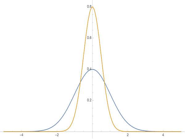
Standard normal distribution (blue) and small-variance normal distribution (orange)
As for the posterior distribution $p(z|x)$, we also assumed it to be a normal distribution. Since we've just argued that $z$ and $x$ are almost in one-to-one correspondence, the same property should apply to the posterior $p(z|x)$ as well — which means the posterior is also a normal distribution with small variance (readers can verify this themselves by examining the encoder's outputs on MNIST). This in turn means that samples drawn from $p(z|x)$ each time are almost identical. Given this, sampling once versus sampling many times makes almost no difference, since the results of each sample are essentially the same. This explains why we can start from equation $(3)$ and, by sampling just a single point, arrive at equation $(4)$ or $(5)$.
The Elegance of the Posterior
We've now given a preliminary explanation for why sampling directly from the prior distribution $q(z)$ doesn't train well, while sampling from the posterior distribution $p(z|x)$ only requires a single point. In fact, using KL divergence to introduce a posterior distribution into a latent-variable model is a remarkably clever trick. In this section, we'll organize these ideas further and present a new example that applies this same principle.
The Prior Behind the Posterior
Readers may feel a bit confused at this point: you're saying that $q(x|z)$ and $p(z|x)$ end up being normal distributions with small variance, but that's just the final result of training. When we're constructing the model, in principle we can't know in advance how small the variances of $q(x|z)$ and $p(z|x)$ will be — so how can we justify sampling just one point from the start?
I think this is actually our prior understanding of the problem. When we decide to train a VAE on a particular dataset $X$, that dataset itself carries strong constraints. For example, the MNIST dataset has 784 pixels, but its true intrinsic dimensionality is far smaller than 784 — most obviously, some border pixels are always zero. MNIST is an extremely small subset relative to the space of all 28×28 images. Similarly, take the poetry-writing bot I wrote about a few days ago: the corpus of "Tang poetry" is a tiny subset relative to the space of all possible sentences. Even the thousand-category ImageNet dataset is just a small subset among the infinite space of possible images.
Given this, we can imagine that the dataset $X$ can be projected into a low-dimensional space (the latent space), where the latent variables correspond one-to-one with the original $X$ data. Readers might have realized: isn't this just an ordinary autoencoder? Indeed — the point is that, in the ordinary autoencoder setting, we can achieve a one-to-one correspondence between latent variables and the original dataset (a perfect one-to-one correspondence would mean the variance of $p(z|x)$ and $q(x|z)$ is zero). Once we then introduce a Gaussian-form prior distribution $q(z)$, roughly speaking, this only amounts to a shift and rescaling of the latent space, so the variance can remain small.
So, we should be guessing in advance that $q(x|z)$ and $p(z|x)$ have small variance, and then letting the model realize this guess. In other words, the operation of "sampling just one point" reflects our prior understanding of the data and the model — it's a prior imposed on the posterior distribution, and we use this prior understanding to steer the model toward matching it.
The overall line of reasoning should be:
1. We start with the raw corpus;
2. By observing the raw corpus, we infer that it can be put in one-to-one correspondence with some latent space;
3. Through the "sample just one" mechanism, we get the model to learn this correspondence.
This section has been a bit rambling — it might even feel somewhat superfluous. I hope I haven't confused readers too much. If it feels muddled, feel free to skip this part.
The Straightforward IWAE
The next example is called the "Importance Weighted Autoencoder" (Importance Weighted Autoencoders]), abbreviated "IWAE." It demonstrates the clever use of the posterior distribution in an even more direct and forthright way, and to some extent can be seen as an upgraded version of VAE.
IWAE starts from equation $(2)$, and rewrites equation $(2)$ by introducing the posterior distribution:
$$\int q(x|z)q(z)dz = \int p(z|x)\frac{q(x|z)q(z)}{p(z|x)}dz=\mathbb{E}_{z\sim p(z|x)}\left[\frac{q(x|z)q(z)}{p(z|x)}\right]\tag{8}$$
This turns equation $(2)$ from sampling from $q(z)$ into sampling from $p(z|x)$. We've already argued that $p(z|x)$ has small variance, so sampling just a few points is enough:
$$\int q(x|z)q(z)dz = \frac{1}{k}\sum_{i=1}^k \frac{q(x|z_i)q(z_i)}{p(z_i|x)},\quad z_1,\dots,z_k\sim p(z|x)\tag{9}$$
Substituting into equation $(2)$ gives
$$q(x|z)=\mathop{\text{argmax}}_{q(x|z)} \mathbb{E}_{x\sim\tilde{p}(x)}\Bigg[\ln\left(\frac{1}{k}\sum_{i=1}^k \frac{q(x|z_i)q(z_i)}{p(z_i|x)}\right)\Bigg],\quad z_1,\dots,z_k \sim p(z|x)\tag{10}$$
This is IWAE. To align with equation $(4),(5)$, we can equivalently rewrite it as
$$\begin{aligned}&q(x|z) = \mathop{\text{argmin}}_{q(x|z),p(z|x)} \mathcal{L}_k,\\ \mathcal{L}_k = \mathbb{E}_{x\sim\tilde{p}(x)}\Bigg[&-\ln\left(\frac{1}{k}\sum_{i=1}^k \frac{q(x|z_i)q(z_i)}{p(z_i|x)}\right)\Bigg],\quad z_1,\dots,z_k \sim p(z|x)\end{aligned}\tag{11}$$
When $k=1$, the expression above is exactly the same as equation $(5)$, so from this perspective, IWAE is an upgraded version of VAE.
Looking at how it's constructed, in equation $(8)$, replacing $p(z|x)$ with any distribution over $z$ is valid; the choice of $p(z|x)$ is only because it has good concentration properties, making sampling convenient. And when $k$ is large enough, in fact the exact form of $p(z|x)$ no longer matters much. This shows that IWAE weakens the role of the encoder model $p(z|x)$, in exchange for an improvement in the generative model $q(x|z)$. This is because in VAE, we assume $p(z|x)$ is normal, which is merely a convenient approximation, and the appropriateness of this approximation also affects the quality of the generative model $q(x|z)$. It can be shown that $\mathcal{L}_k$ gets closer to the lower bound $-\mathbb{E}_{x\sim \tilde{p}(x)} \left[\ln \tilde{p}(x)\right]$ than $\mathcal{L}$ does, so the resulting generative model is of higher quality.
Intuitively, in IWAE, how good the approximation $p(z|x)$ is no longer matters as much, which allows for a better generative model. The trade-off is that the quality of the encoding model degrades — again because the importance of $p(z|x)$ is reduced, so the model no longer focuses as much effort on training $p(z|x)$. So if our goal is to obtain a good encoder, IWAE is not the way to go.
There's also a related work, Tighter Variational Bounds are Not Necessarily Better], which reportedly improves both encoder and decoder quality simultaneously, though I haven't fully understood it yet.
The Magic of Reparameterization
If the introduction of the posterior distribution successfully sketches out the overall blueprint of VAE, then the reparameterization trick is the "finishing touch" that brings the whole picture to life.
Earlier we said that by introducing the posterior distribution, VAE shifts sampling from the loose standard normal distribution $q(z)$ to the compact normal distribution $p(z|x)$. However, although both are normal distributions, their meanings are quite different. Let's first write
$$p(z|x)=\frac{1}{\prod\limits_{k=1}^d \sqrt{2\pi \sigma_{(k)}^2(x)}}\exp\left(-\frac{1}{2}\left\Vert\frac{z-\mu(x)}{\sigma(x)}\right\Vert^2\right)\tag{12}$$
That is, the mean and variance of $p(z|x)$ are both quantities produced by models we need to train.
Now imagine: once the model reaches this point and computes $\mu(x)$ and $\sigma(x)$, we can then construct the normal distribution and sample from it. But what comes out of the sampling? It's a vector — and one whose relationship to $\mu(x)$ and $\sigma(x)$ is not apparent, so it's effectively treated as a constant vector. Taking its derivative gives nothing, and so in gradient descent, we get no feedback whatsoever to update $\mu(x)$ and $\sigma(x)$.
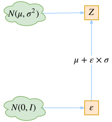
The reparameterization trick
This is where the reparameterization trick makes its grand entrance, telling us bluntly:
$$z = \mu(x) + \varepsilon \times \sigma(x),\quad \varepsilon\sim \mathcal{N}(0,I).$$
Nothing could be more concise. It looks like a tiny transformation, but it explicitly reveals the relationship between $z$ and $\mu(x),\sigma(x)$! Now taking the derivative of $z$ is no longer zero, and $\mu(x),\sigma(x)$ can finally receive the feedback that belongs to them. At this point, everything is in place for the model, and all that remains is to write the code.
Clearly, "reparameterization" is nothing short of a killer move.
Watering Down This Post
Rambling on and on — another watered-down post is done.
This post has mainly tried to clarify some finer details following up on VAE, in particular how VAE cleverly resolves the sampling problem (and thereby the training problem) by introducing the posterior distribution, and along the way introduced IWAE.
Aiming for intuitive understanding inevitably sacrifices some rigor — you can't have both at once. So, for any flaws in this article, I ask expert readers for their forbearance, and welcome any criticism or suggestions.
Translated automatically with claude-sonnet-5; all equations are reproduced verbatim from the source. Copyright remains with the original author.