Why Is the Lebesgue Integral Better Than the Riemann Integral?

为什么勒贝格积分比黎曼积分强？ 苏剑林 · 2016-11-16 · Mathematics integral analysis measure

Anyone who has studied real analysis will know of something called the Lebesgue integral, said to be an improved version of the Riemann integral. Even though "learning real analysis ten times over will chill your heart before you even reach functional analysis," when we were studying real analysis we were usually completely lost — but by the end, thanks to our teachers' "irrigation," we absorbed a few conclusions by osmosis, such as "a Riemann-integrable function (on a finite interval) is also Lebesgue-integrable." Put plainly, this amounts to "the Lebesgue integral is stronger than the Riemann integral." So the question is: stronger in what sense? And why is it stronger?

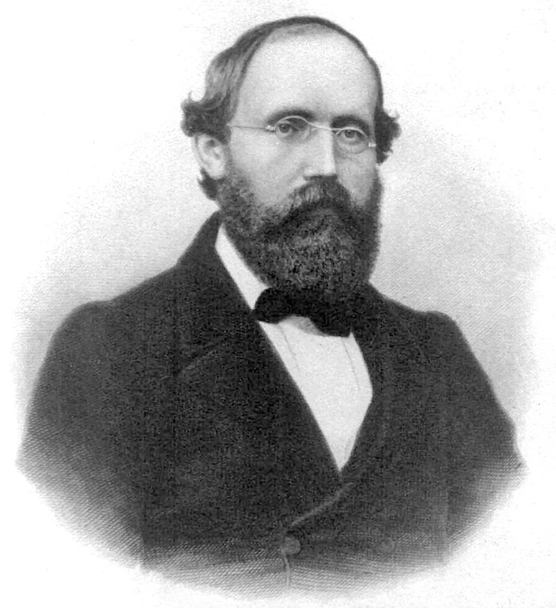
Riemann

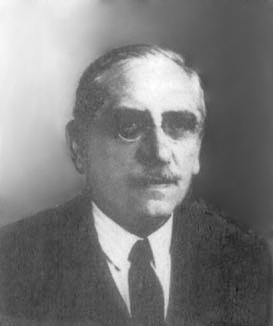
Lebesgue

I never really understood this question when I was studying real analysis, and I let it sit for a long time afterward, until recently, after carefully reading Revisiting Calculus, I finally got some sense of it. Incidentally, Professor Qi Minyou's Revisiting Calculus is truly excellent and well worth reading.

Born of the Same Root, Why Such Rivalry?

Anyone who has studied real analysis knows that, as two different theories describing integration, the most obvious difference between the Lebesgue integral and the Riemann integral is: the Riemann integral partitions the domain, while the Lebesgue integral partitions the range. At first glance, it looks as if Lebesgue is deliberately doing the opposite of Riemann — "you want to partition the domain? Well, I won't; I insist on partitioning the range instead."

So what's really going on? Is it really just rivalry for rivalry's sake? Not at all — partitioning the range genuinely helps overcome a shortcoming of the Riemann integral. Why does partitioning the range do better than partitioning the domain? The popular explanation goes like this: the Riemann integral partitions the domain, but for a function that oscillates wildly, no matter how finely you partition, the oscillation within each tiny subinterval can remain severe (the classic example being the Dirichlet function), in which case the Riemann integral simply cannot be defined. In other words, the Riemann integral only works for functions that are locally well-behaved. The Lebesgue integral, on the other hand, partitions the range, so that within a small subinterval of the range there can be no large oscillation — the range has already been pinned down, leaving the function no room to oscillate. This is why it can integrate functions that oscillate very badly.

Others Laugh at My Madness; I Laugh at Their Blindness

Lebesgue speaks up: "What you're saying is somewhat on the right track, but it still misses my real intent. Let me be clear — I was never trying to oppose the great Riemann..." (Purely my own invention ^_^)

In fact, the shortcomings of the Riemann integral can be traced back to the "method of exhaustion" of ancient Greece two thousand years ago. To find the area of a circle, for instance, one used circumscribed regular $n$-gons and inscribed regular $n$-gons to get upper and lower bounds on the area, and then took the limit and found that the two bounds coincided — hence that was the area of the circle. In other words, to find the area of an irregular shape, one splits it into pieces, approximates each piece by a familiar shape (rectangle, triangle), sums up the approximate areas, and finally takes the limit as the partition is refined. The whole process is: finite partition — approximate summation — take the limit.

The problem lies precisely in "finite partition"! To obtain an upper bound for the area of a shape, we need to cover it with finitely many simple shapes; to get a lower bound, we need finitely many simple shapes covered by the shape. Either way, it's always "finitely many." This finiteness is fine for continuous intervals, but it fails for general point sets. Take, for example, the set of rational numbers within $[0,1]$ — imagine on the number line the set of all rational points in the interval $[0,1]$, and consider its length. Anyone who has studied set theory knows that the cardinality of the real numbers in the interval $[0,1]$ is uncountable, while the rationals are countable — that is, there are vastly more reals than rationals. So if we take the length of the set of all real points in the interval $[0,1]$ to be 1, then naturally the length of the set of all rational points in the interval $[0,1]$ ought to be 0. However, the finite partitioning used by the Riemann integral cannot deliver this conclusion.

If we try to cover all the rational numbers in the interval $[0,1]$ with finitely many intervals (covering to get an upper bound), then, because the rationals are dense, we can imagine that the total length of these finitely many intervals cannot be less than 1 — that is, the upper bound on the total length of all the rationals in the interval $[0,1]$ cannot be less than 1. Yet, because every interval contains irrational numbers, the rationals cannot cover any interval (no matter how small its length), and from this angle, the lower bound on the total length of the rationals cannot exceed 0. This shows the result does not converge! This is exactly the problem caused by finite partitioning.

Lebesgue, being clever, abandoned finite partitioning from the very start and instead used countable partitioning from the outset to define measure. Here I won't reproduce the rigorous textbook language, just the general idea: taking the one-dimensional case as an example, if a subset of the real numbers can be covered by countably many intervals, the total length of those intervals gives an upper bound on its measure; if it can cover countably many intervals, their total length gives a lower bound on its measure; and if the limits of the upper and lower bounds coincide, the set is measurable.

Great Wisdom Often Looks Like Foolishness, Great Skill Often Looks Clumsy

Once we have countable partitioning, we can try to improve the Riemann integral. With countable partitioning available, we can split a function into several parts for separate treatment — say, into "normal" points and "abnormal" points, with the abnormal part further subdivided into a first kind of abnormality, a second kind, and so on, handled one by one — and countable partitioning is the foundation that makes this possible. For instance, if we want to pick out all the rational points while keeping the total interval length arbitrarily small, we must use countably many intervals; finitely many will not do.

But then another question arises: how do we distinguish "normal" from "abnormal" points? For the Riemann integral, the abnormal points are exactly the points of severe oscillation. In other words, we need to look at the range! This is where another stroke of Lebesgue's ingenuity comes in: rather than classifying the abnormal points of the Riemann integral one by one, just partition the range directly.

At first glance, partitioning the range seems like a very unintuitive, clumsy approach, because it makes the corresponding pieces of the domain more complicated. In fact, this is exactly the "great wisdom that looks like foolishness," because countable partitioning has already been set up beforehand, and it can handle domains of arbitrary complexity. So, by combining "countable partitioning" with "range partitioning," the theory called the Lebesgue integral took shape, and the rest is just theoretical detail. Incidentally, because it relies on countable partitioning, the Lebesgue integral naturally has countable additivity, whereas the corresponding Riemann integral only has finite additivity.

From this discussion we can see that Lebesgue measure and the Lebesgue integral can handle cases with countably many abnormal points (discontinuities). It's therefore clear that when the number of abnormal points becomes uncountable, both Lebesgue measure and the Lebesgue integral fail. So, to construct an example that is not Lebesgue-measurable, one must push the number of abnormal points up to uncountable — and this is exactly how the non-measurable "Vitali set" is constructed. Starting from the fact that the reals are uncountable while the rationals are countable, and using the rationals as a reference, one divides $[0,1]$ of the reals into countably many pieces, each of which is uncountable. But the question is: what is the measure of each piece? If it's 0, how can countably many zeros sum to 1? And if it's not 0, then countably many positive numbers summing to 1 is even more impossible. Either way, countable additivity fails.

Nothing Rigid Lasts, Nothing Yielding Holds Forever — Extremes Reverse Themselves

From this it does seem that the Lebesgue integral is indeed stronger than the Riemann integral, since it was designed from the outset precisely to target the Riemann integral's "Achilles' heel."

In life, we often find that being too purpose-driven backfires. Since the Lebesgue integral is so pointedly designed to "counter" the Riemann integral, might it not also have some drawbacks that the Riemann integral doesn't have?

First, it's quite clear that linearity becomes much less obvious for the Lebesgue integral — a great deal of effort is spent proving that

$$\int_a^b f(x)dx + \int_a^b g(x)dx=\int_a^b [f(x)+g(x)]dx$$

whereas in the Riemann integral this is almost trivially true. This is perhaps one reason why introductory calculus courses always use the Riemann definition — it's simply more intuitive.

There are also some drawbacks that cannot be overcome. Inspired by the Dirichlet function, it's easy to construct examples that are Riemann non-integrable but Lebesgue integrable. Is the reverse possible? The answer is yes!

We can already spot the issue in the "countable partitioning" of the Lebesgue integral mentioned earlier. The Lebesgue integral allows approximation by countably many intervals from the very start, and then computes the sum of the function's values over these countably many intervals. Because the countable partition and the ensuing summation have no inherent order, this summation process is order-independent. We know that a series that can be summed without regard to order is exactly what we call an absolutely convergent series. So we can sense that the Lebesgue integral must be (in the Riemann sense) absolutely convergent.

However, many practically useful integrals are not absolutely convergent. For example, the integral

$$\int_{-\infty}^{+\infty} \frac{\sin x}{x}dx$$

is only conditionally convergent, not absolutely convergent, and so it is not integrable in the Lebesgue sense! Whereas for the Riemann integral, if we understand it as

$$\lim_{N\to\infty}\int_{-N}^{+N} \frac{\sin x}{x}dx$$

we obtain a meaningful result. There's something almost ironic here: "countable partitioning" was originally introduced to fix a weakness of the Riemann integral, but here it turns into a weakness of its own. It seems that "things carried to an extreme reverse themselves," and there really is no perfect, catch-all solution. Consider the following example as well.

Return to Simplicity, Never Forget the Original Intent

Let's talk about probability theory, and consider the following question:

If we randomly pick a number from the natural numbers, what is the probability of picking 1?

Obviously 0? Intuitively we'd say 0, but according to the modern axiomatic definition, this probability doesn't exist at all!! It cannot be defined!!

Let's look at the axiomatic definition of probability:

For every event A, if the function P(A) satisfies the following conditions, then P(A) is the probability of A:
1. Non-negativity: P(A) is non-negative;
2. Normalization: for the certain event S, P(S) = 1;
3. Countable additivity: the probability of the union of mutually exclusive events equals the sum of their probabilities.

The first two conditions aren't the key issue — it's the third, countable additivity! If we say the probability of picking 1 is 0, then the probability of picking 2 is also 0, and likewise for every given natural number — and countably many zeros still sum to 0. So the probability of picking some natural number would be 0, not 1! That is, countable additivity fails.

So it would seem that we simply cannot talk about probability on a countable set — which would mean that the mathematicians working in "probabilistic number theory," a branch of number theory, have been talking pure nonsense all along... Is that really so?

Where does the axiomatic definition of probability — and countable additivity in particular — come from? Compare it with the axiomatic definition of Lebesgue measure, and you'll find that, aside from a difference in wording, they are almost identical; countable additivity is also a requirement of measure! In fact, probability defined this way is essentially a kind of Lebesgue measure — or rather, the definition of probability is essentially borrowed wholesale from the definition of measure. And the example above shows that countable additivity really is a thing we both love and hate.

Yet we still feel the need to discuss probability on the set of natural numbers — so what do we do? Probabilistic number theory handles this by first discussing things within the range of natural numbers not exceeding $N$, and then letting $N$ tend to positive infinity. Well — isn't that exactly back to the Riemann approach of finite partitioning followed by taking a limit...

It seems that, in the end, we really can't "overthrow Riemann" after all...