【Understanding Riemannian Geometry】5. Riemann Curvature

【理解黎曼几何】5. 黎曼曲率 苏剑林 · 2016-10-18 · Mathematics geometry curvature riemannian geometry

Now let's turn our attention to Riemann curvature. Broadly speaking, Riemann curvature offers a scheme by which someone living inside a space can compute how curved that space is, purely from within it. As the saying goes, "one cannot see the true face of Mount Lu while standing inside it," or "the onlooker sees clearest, the player is lost in the game." Being able to detect whether a space is curved while standing inside it is a remarkable feat—it's as if we had transcended our own space and climbed up into a higher-dimensional one to look down from above. Truly, "as far as the heart reaches, so far does the road, so far does the world."

If you look at things from the vantage point of a higher-dimensional space, it's easy to spot curvature. For example, suppose there is a geodesic in a curved space; viewed from the higher-dimensional embedding space, it appears as a curve, and one can compute its curvature and so on. But viewed from within the original space, it looks straight—a geodesic is, after all, the generalization of the concept of a straight line. So this route cannot possibly reveal the curvature of the space; we need some more roundabout approach. It might not be obvious at first, but once several different routes converge on the same conclusion, it starts to feel self-evident.

How can we better derive Riemann curvature, in a way that makes the essential difference between curved and flat space manifest? I spent quite a long time thinking about this, consulting a number of reference books (Gravitation and Spacetime, Field Theory, Theory of Gravitation, etc.), and comparing several ways of deriving Riemann curvature. Let me summarize them briefly below. more

The Order of Differentiation Matters

In most textbooks on tensor analysis or Riemannian geometry, Riemann curvature is derived by examining the difference that arises from the order of second covariant derivatives:

$$A^{\mu}_{;\alpha;\beta}-A^{\mu}_{;\beta;\alpha}=-R^{\mu}_{\nu\alpha\beta}A^{\nu} \tag{40} $$

From this one can extract the Riemann curvature tensor $R^{\mu}_{\nu\alpha\beta}$. This is indeed a satisfyingly direct route, but its geometric meaning is not obvious—it's hard to see how it reflects whether space is curved or flat. Moreover, we haven't yet defined the second covariant derivative (after one covariant differentiation you get two indices, i.e., something like a matrix rather than a vector, and defining higher-order covariant derivatives requires some further technical bookkeeping); this definition is essentially pure algebraic manipulation, which isn't especially meaningful for our purposes here, so we won't define it. Readers can simply consult a textbook directly, and we won't dwell further on this approach.

An Encounter in Curved Space

There is also a way of deriving Riemann curvature via geodesic deviation (which, in general relativity, corresponds to tidal forces). This is a scheme with a very clear geometric and physical meaning, though the computations involved are somewhat tedious. The main idea is as follows. Consider the geodesic equation

$$\frac{d^2 x^{\mu} }{ds^2}+\Gamma_{\alpha\beta}^{\mu}(x) \frac{d x^{\alpha} }{ds}\frac{d x^{\beta} }{ds}=0 \tag{41} $$

Suppose there is another geodesic $x(s)+\delta x(s)$, satisfying the equation

$$\frac{d^2 (x^{\mu} + \delta x^{\mu}) }{ds^2}+\Gamma_{\alpha\beta}^{\mu}(x+\delta x) \frac{d (x^{\alpha}+\delta x^{\alpha}) }{ds}\frac{d (x^{\beta}+\delta x^{\beta}) }{ds}=0 \tag{42} $$

Assuming both $\delta x$ and $d\delta x/ds$ are infinitesimal, subtracting the two equations gives

$$\frac{d^2 \delta x^{\mu}}{ds^2}+\frac{\partial \Gamma_{\alpha\beta}^{\mu}}{\partial x^{\nu}}\delta x^{\nu} \frac{d x^{\alpha} }{ds}\frac{d x^{\beta}}{ds}+2\Gamma_{\alpha\beta}^{\mu}\frac{d \delta x^{\alpha} }{ds}\frac{d x^{\beta}}{ds}=0 \tag{43} $$

where $\delta x$ is called the geodesic deviation, known in Riemannian geometry as the "Jacobi vector field." The above form is already simple enough, but we prefer to write it in terms of covariant derivatives, since the covariant derivative is the appropriate notion of derivative in curved space. We already defined the derivative along a geodesic, $\frac{DA^{\mu}}{Ds}$; repeating this once more gives us the second derivative along the geodesic, $\frac{D^2 A^{\mu}}{Ds^2}=\frac{D}{Ds}\left(\frac{DA^{\mu}}{Ds}\right)$, which is straightforward to obtain. Since this isn't the approach we're most interested in here, we won't write out the explicit form of $\frac{D^2 A^{\mu}}{Ds^2}$—readers can work it out themselves. After carrying out the computation, one finds

$$\frac{D^2 \delta x^{\mu}}{Ds^2}=-R^{\mu}_{\nu\alpha\beta}\delta x^{\alpha}\frac{dx^{\nu}}{ds}\frac{dx^{\beta}}{ds} \tag{44} $$

and here the curvature tensor $R^{\mu}_{\nu\alpha\beta}$ makes its appearance. Mathematically, a nonzero $R^{\mu}_{\nu\alpha\beta}$ reflects the non-uniformity of the distribution of geodesics, which is one manifestation of curved space.

This scheme reminds me of Jimmy Liao's comic Turn Left, Turn Right, about a man and a woman who each habitually walk in opposite directions—he always turns left, she always turns right—so it would seem they can never meet. But one day they meet at a round fountain: walking away from each other at one end of the circle, they eventually meet again at the other end. In curved space, such as on the surface of a sphere, even two "parallel" lines have the chance to intersect. This actually reveals something deeper and more interesting about "curvature": it endows our world with far more possibilities.

The Change Upon "Wandering" Back

Finally, there is a scheme based on analyzing how a vector changes after being parallel-transported around a closed loop, which we will examine in detail here. In fact, it is equivalent to the geodesic-deviation approach, but its geometric meaning is more transparent, which helps in deriving deeper results. It shows that if a vector "wanders" around a loop and comes back to where it started, it need not be the same vector it was originally. The figure below illustrates this clearly.

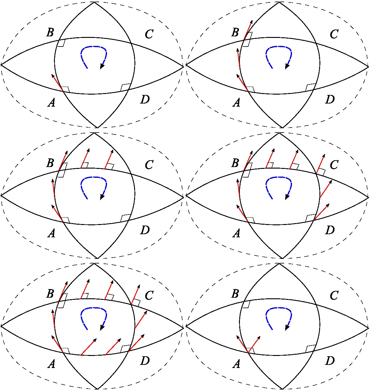Parallel transport

Suppose at $x^{\mu}$ there is an arbitrary vector $A^{\mu}$. Starting from $x^{\mu}$, we parallel-transport it first by an infinitesimal amount $dx^{\mu}$, then by an infinitesimal amount $\delta x^{\mu}$, then by an infinitesimal amount $-dx^{\mu}$, and finally by an infinitesimal amount $-\delta x^{\mu}$—that is, we walk once around an infinitesimal parallelogram and return to the starting point:

$$x^{\mu}\to x^{\mu}+dx^{\mu}\to x^{\mu}+dx^{\mu}+\delta x^{\mu}\to x^{\mu}+\delta x^{\mu}\to x^{\mu}$$

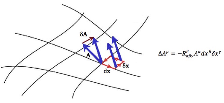Parallel transport

Let's compute step by step how $A^{\mu}$ changes during this transport. Going from $x^{\mu}$ to $x^{\mu}+dx^{\mu}$, $A^{\mu}$ becomes

$$A^{\mu}-\Gamma^{\mu}_{\alpha\beta}(x) A^{\alpha}dx^{\beta} \tag{45} $$

Then, going from $x^{\mu}+dx^{\mu}$ to $x^{\mu}+dx^{\mu}+\delta x^{\mu}$, $A^{\mu}$ becomes

$$\begin{aligned}&A^{\mu}-\Gamma^{\mu}_{\alpha\beta}(x) A^{\alpha}dx^{\beta}-\Gamma^{\mu}_{\nu\gamma}(x+dx) \left[A^{\nu}-\Gamma^{\nu}_{\alpha\beta}(x) A^{\alpha}dx^{\beta}\right]\delta x^{\gamma}\\ =&A^{\mu}-\Gamma^{\mu}_{\alpha\beta}(x) A^{\alpha}dx^{\beta}-\Gamma^{\mu}_{\nu\gamma}(x) A^{\nu} \delta x^{\gamma} \\ &\quad- \frac{\partial \Gamma^{\mu}_{\nu\gamma}(x)}{\partial x^{\beta}} A^{\nu} dx^{\beta} \delta x^{\gamma} + \Gamma^{\mu}_{\nu\gamma}(x) \Gamma^{\nu}_{\alpha\beta}(x) A^{\alpha} dx^{\beta}\delta x^{\gamma} \end{aligned} \tag{46} $$

Here we keep terms up to second order only.

Similarly, if we consider the change brought about by the path $x^{\mu}\to x^{\mu}+\delta x^{\mu}\to x^{\mu}+dx^{\mu}+\delta x^{\mu}$, we need only swap $dx$ and $\delta x$

$$\begin{aligned}&A^{\mu}-\Gamma^{\mu}_{\alpha\beta}(x) A^{\alpha}\delta x^{\beta}-\Gamma^{\mu}_{\nu\gamma}(x) A^{\nu} d x^{\gamma} \\ &\quad- \frac{\partial \Gamma^{\mu}_{\nu\gamma}(x)}{\partial x^{\beta}} A^{\nu} \delta x^{\beta} d x^{\gamma} + \Gamma^{\mu}_{\nu\gamma}(x) \Gamma^{\nu}_{\alpha\beta}(x) A^{\alpha} \delta x^{\beta} d x^{\gamma}\end{aligned} \tag{47} $$

Then, quite naturally, the change caused by path $x^{\mu}+dx^{\mu}+\delta x^{\mu}\to x^{\mu}+\delta x^{\mu}\to x^{\mu}$ is the negative of the above expression. So the net change over the whole closed path $x^{\mu}\to x^{\mu}+dx^{\mu}\to x^{\mu}+dx^{\mu}+\delta x^{\mu}\to x^{\mu}+\delta x^{\mu}\to x^{\mu}$ is the difference between the two expressions. Rearranging the summation indices and taking the difference, we readily obtain

$$\label{bihelujingbianhua}\begin{aligned}\Delta A^{\mu} =&-\left(\frac{\partial \Gamma^{\mu}_{\alpha\gamma}}{\partial x^{\beta}}-\frac{\partial \Gamma^{\mu}_{\alpha\beta}}{\partial x^{\gamma}}+\Gamma^{\mu}_{\nu\beta}\Gamma^{\nu}_{\alpha\gamma}-\Gamma^{\mu}_{\nu\gamma}\Gamma^{\nu}_{\alpha\beta}\right)A^{\alpha} dx^{\beta}\delta x^{\gamma}\\ =&-R^{\mu}_{\alpha\beta\gamma} A^{\alpha} dx^{\beta}\delta x^{\gamma}\end{aligned} \tag{48} $$

where

$$R^{\mu}_{\alpha\beta\gamma}=\frac{\partial \Gamma^{\mu}_{\alpha\gamma}}{\partial x^{\beta}}-\frac{\partial \Gamma^{\mu}_{\alpha\beta}}{\partial x^{\gamma}}+\Gamma^{\mu}_{\nu\beta}\Gamma^{\nu}_{\alpha\gamma}-\Gamma^{\mu}_{\nu\gamma}\Gamma^{\nu}_{\alpha\beta} \tag{49} $$

is precisely the defining expression for the Riemann curvature tensor. It carries four indices, making it a truly "grand" quantity.

In a Nutshell

These three different ways of deriving the Riemann curvature tensor each reveal, from their own angle, the distinction between curved and flat space: in flat space, the order of covariant differentiation can be swapped, while in curved space it cannot; in flat space, geodesics are distributed uniformly and linearly, while in curved space they are not; and in flat space, a vector that "wanders" around a loop and returns is unchanged, while in curved space, after such a journey, the vector may no longer be what it originally was.