【Understanding Riemannian Geometry】4. Connections and Covariant Derivatives

【理解黎曼几何】4. 联络和协变导数 苏剑林 · 2016-10-16 · Mathematics geometry analysis riemannian geometry

Vectors and Connections

Once we've built our own coordinate system at our location, we can make all sorts of measurements. Some of the results are scalars — temperature, mass — and these are the same no matter what coordinate system you use. Sometimes, however, we measure vectors: velocity, acceleration, force, and so on. These are also objective entities, but since the measurement result is expressed via the components in a coordinate system, changing coordinates will completely change the components.

If everyone at every location used the same coordinates, there'd be no controversy. But as we've emphasized repeatedly, people at different locations may, for various reasons, use different coordinate systems. So when we write down a vector $A^{\mu}$, strictly speaking we should note that it was measured at location $\boldsymbol{x}$: $A^{\mu}(\boldsymbol{x})$, and we're only allowed to drop this notation when it causes no ambiguity.

At this point, we're already able to do some computation. For instance, suppose $A^{\mu}$ is measured at $\boldsymbol{x}$, and the formula for the norm at $\boldsymbol{x}$ is $ds^2 = g_{\mu\nu} dx^{\mu} dx^{\nu}$; then the norm of $A^{\mu}$ is $\sqrt{g_{\mu\nu} A^{\mu}A^{\nu}}$, which is an objective entity.

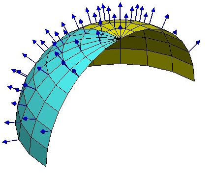As shown, one can set up different local coordinate systems at every point on a sphere; at the very least, the vertical axes of these coordinate systems point in different directions. more

Sometimes we want to compare two vectors measured at different locations, which involves taking a difference. In particular, since the coordinate systems at different locations differ, directly subtracting the components of two vectors measured at different locations is meaningless. It's like saying we can't conclude that "5 US dollars − 5 Chinese yuan = (5−5) = 0." But that particular example is just a matter of mismatched units — if we used the same unit, there'd be no problem. However, a vector measurement depends not only on units but also on the coordinate system. For instance, suppose a plane flies from China to the United States. At some point over China, its measured velocity is $(300,300,300)$; at some point over the US, its measured velocity is also $(300,300,300)$, with both measured in "km/h." But the measurement over China was made by a Chinese observer, and the one over the US by an American observer. As we all know, the US and China sit at nearly opposite sides of the globe, so the local coordinate systems they set up are certainly different. Hence we cannot conclude that the plane's velocity difference between the two locations is $(300-300,300-300,300-300)=(0,0,0)$ — because direction matters too!

Put plainly, the root of the problem is that different locations use different coordinate systems — different unit lengths, different axis orientations, and so on. So we need to transform the vector components from one location's coordinates into another location's coordinates before we can compare them. Here, we'll only consider the transformation between two locations separated by an infinitesimal distance, $\boldsymbol{x}$ and $\boldsymbol{x}+d\boldsymbol{x}$ — that is, how to express a vector $A^{\mu}(\boldsymbol{x}+d\boldsymbol{x})$ measured at $\boldsymbol{x}+d\boldsymbol{x}$ (which has its own coordinate system at $\boldsymbol{x}+d\boldsymbol{x}$) in terms of the coordinate system at $\boldsymbol{x}$. Clearly, this involves a transformation matrix, so the key task is to determine this matrix.

How do we find this matrix? Imagine placing a test vector at $\boldsymbol{x}$, and then moving it over to $\boldsymbol{x}+d\boldsymbol{x}$ to see what it becomes. With enough test vectors, we can pin down the transformation matrix. So we need a set of the most natural test vectors to serve as our reference — and we already know of one objective entity that provides exactly this: the geodesic. In fact, geodesics give us the most natural reference object possible; nothing could be more natural. We can rewrite the geodesic equation as

$$d\left(\frac{d x^{\mu} }{ds}\right)=-\Gamma_{\alpha\beta}^{\mu} \frac{d x^{\alpha} }{ds}d x^{\beta} \tag{28} $$

This formula means: if we have a unit vector $\frac{dx^{\mu}}{ds}$ at the current location $\boldsymbol{x}$, and it moves forward along the geodesic direction by $d\boldsymbol{x}$, then the change in the unit vector $\frac{dx^{\mu}}{ds}$ is $d\left(\frac{d x^{\mu} }{ds}\right)$, which also equals $-\Gamma_{\alpha\beta}^{\mu} \frac{d x^{\alpha} }{ds}d x^{\beta}$, i.e.,

$$\frac{dx^{\mu}}{ds}\quad\to\quad \frac{dx^{\mu}}{ds}-\Gamma_{\alpha\beta}^{\mu} \frac{d x^{\alpha} }{ds}d x^{\beta} \tag{29} $$

Then the coordinate transformation matrix (the Jacobian) from $\boldsymbol{x}$ to $\boldsymbol{x}+d\boldsymbol{x}$ is

$$\frac{\partial\left(\frac{dx^{\mu}}{ds}-\Gamma_{\alpha\beta}^{\mu} \frac{d x^{\alpha} }{ds}d x^{\beta}\right)}{\partial \frac{dx^{\nu}}{ds}}=\delta_{\nu}^{\mu}-\Gamma_{\nu\beta}^{\mu} d x^{\beta} \tag{30} $$

And conversely, the coordinate transformation matrix from $\boldsymbol{x}+d\boldsymbol{x}$ to $\boldsymbol{x}$ is

$$\label{lianluo}\delta_{\nu}^{\mu}+\Gamma_{\nu\beta}^{\mu} d x^{\beta} \tag{31} $$

Looking at it this way, the coefficient $\Gamma_{\alpha\beta}^{\mu}$ links the coordinates at the two locations $\boldsymbol{x}$ and $\boldsymbol{x}+d\boldsymbol{x}$, which makes it entirely fitting to call it the "connection coefficient."

Now that we know how the coordinates transform, we can readily see that if we take $A^{\mu}(\boldsymbol{x}+d\boldsymbol{x})$ and measure it at location $\boldsymbol{x}$, the result will be

$$\left(\delta_{\nu}^{\mu}+\Gamma_{\nu\beta}^{\mu} d x^{\beta}\right) A^{\nu}(\boldsymbol{x}+d\boldsymbol{x})=A^{\mu}(\boldsymbol{x}+d\boldsymbol{x})+\Gamma_{\nu\beta}^{\mu} A^{\nu}(\boldsymbol{x}+d\boldsymbol{x}) d x^{\beta} \tag{32} $$

Covariant Derivative

As mentioned earlier, we sometimes need to take the difference of vectors, and in the discussion of connections we've already worked out the coordinate transformation between two infinitesimally close locations, giving us the result of equation $(32)$: if we take $A^{\mu}(\boldsymbol{x}+d\boldsymbol{x})$ and measure it at location $\boldsymbol{x}$, the result will be

$$A^{\mu}(\boldsymbol{x}+d\boldsymbol{x})+\Gamma_{\nu\beta}^{\mu} A^{\nu}(\boldsymbol{x}+d\boldsymbol{x}) d x^{\beta} \tag{33} $$

Now we can directly take the difference, since both vectors are now measured at the same location.

$$A^{\mu}(\boldsymbol{x}+d\boldsymbol{x})+\Gamma_{\nu\beta}^{\mu} A^{\nu}(\boldsymbol{x}+d\boldsymbol{x}) d x^{\beta}-A^{\mu}(\boldsymbol{x}) \tag{34} $$

We can study the limiting case:

$$\lim_{d\boldsymbol{x} \to 0} \frac{A^{\mu}(\boldsymbol{x}+d\boldsymbol{x})+\Gamma_{\nu\beta}^{\mu} A^{\nu}(\boldsymbol{x}+d\boldsymbol{x}) d x^{\beta}-A^{\mu}(\boldsymbol{x})}{dx^{\beta}} \tag{35} $$

It's not hard to show that the result is

$$\frac{\partial A^{\mu}}{\partial x^{\beta}}+\Gamma_{\nu\beta}^{\mu} A^{\nu} \tag{36} $$

This is called the covariant derivative of the vector $A^{\mu}$, denoted

$$A^{\mu}_{;\beta}=\frac{\partial A^{\mu}}{\partial x^{\beta}}+\Gamma_{\nu\beta}^{\mu} A^{\nu} \tag{37} $$

And naturally, the following quantity is called the covariant differential:

$$D A^{\mu}=dA^{\mu}+\Gamma_{\nu\beta}^{\mu} A^{\nu}dx^{\beta} \tag{38} $$

If we divide by the line element $ds$, we obtain the differential

$$\frac{D A^{\mu}}{Ds}=\frac{dA^{\mu}}{ds}+\Gamma_{\nu\beta}^{\mu} A^{\nu}\frac{dx^{\beta}}{ds} \tag{39} $$

We can see that the result depends on the choice of curve $x^{\beta}$; when we choose it to be a geodesic, the above expression is called the geodesic derivative (differentiation along a geodesic).

Looking back over the whole derivation, the starting point for deriving the covariant derivative is this: directly subtracting the components of vectors at two different locations is meaningless; if necessary, we must transform the vector from one location to the other. Taking the limiting case then yields the covariant derivative. The covariant derivative is a derivative defined with genuine geometric meaning in space, and is therefore itself an objective entity.

In typical treatments of tensor analysis or Riemannian geometry, the covariant derivative is derived in many different ways. Some textbooks take the following approach: since we already know the explicit form of the gradient in Cartesian coordinates, we start from Cartesian coordinates and use the transformation laws to obtain the derivative in other coordinate systems. This seems reasonable at first glance, but it actually implicitly assumes flat space — that is, although curvilinear coordinates are used, it's assumed one can transform back to Cartesian coordinates via some change of variables; otherwise the approach doesn't hold. This means the space is flat, and the fact that curved space happens to give the same result is, in a sense, mere coincidence. If one applies the same line of reasoning to derive the Riemann curvature, the result will identically vanish — because the space was flat to begin with.

There are other ways of deriving it as well. On the whole, I feel that most approaches, however you look at them, aren't "geometric enough" — they're more a matter of algebraic manipulation. Here I've tried to take an approach that stays as geometric as possible.