Understanding Riemannian Geometry: 3. Geodesics

【理解黎曼几何】3. 测地线 苏剑林 · 2016-10-15 · Mathematics geometry riemannian geometry calculus of variations

Geodesics

The Riemannian metric shouldn't be too hard to grasp — in differential geometry textbooks we've already learned about the "first fundamental form" of a surface. In fact, the two are the same thing, just viewed from different angles: differential geometry treats a surface as a two-dimensional subset of three-dimensional space, whereas Riemannian geometry studies the geometry of the two-dimensional surface intrinsically, on its own terms.

What is geometry actually concerned with? In fact, geometry is concerned with "objective entities" that are independent of transformations (or, things that remain invariant under transformations) — this is essentially the definition of geometry. According to Klein's Erlangen Program, geometry is the study of properties that remain invariant under some (group of) transformations. If we restrict the transformations to rigid motions (translation, rotation, reflection), we get Euclidean geometry; if the transformations are general linear ones, we get affine geometry. Riemannian geometry, meanwhile, is concerned with objective entities that are independent of all coordinate choices. For example, suppose I have a vector with a fixed direction and magnitude: in Cartesian coordinates it is $(1, 1)$, and in polar coordinates it is $(\sqrt{2}, \pi/4)$. Although the components differ between the two coordinate systems, both refer to the very same vector. In other words, the vector itself is an objectively existing entity, independent of whatever coordinates we choose to describe it. Algebraically speaking, as long as two descriptions can be obtained from each other via some coordinate transformation, we regard them as the same object.

So, when studying Riemannian geometry, it's always helpful to think in terms of "objective entities."

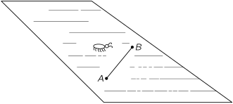Geodesic in the plane

Once we have a metric, we can quite naturally introduce the entity known as the "geodesic." Narrowly speaking, it is the shortest curve between two points — a generalization of the concept of a straight line segment in flat space (the actual geodesic need not be the shortest one, but let's not worry about that detail for now; it doesn't stop us from understanding it, since a geodesic is at least locally the shortest curve). It's not hard to see that once two points are fixed, the shortest curve between them is determined regardless of which coordinates we use — so this is clearly an objective entity. A simple analogy: no matter how we change coordinates, the extremal points on the graph of a function $f(x)$ are always fixed — whether you transform it or not, they're right there, unmoved. more

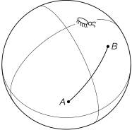Geodesic on a sphere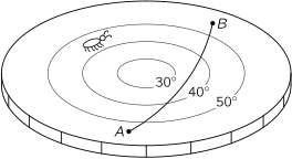Geodesic on an isothermal surface

Mathematically, the distance between two points $\boldsymbol{x}^1$ and $\boldsymbol{x}^2$ is naturally given by

$$s = \int_{\boldsymbol{x}^1}^{\boldsymbol{x}^2} ds = \int_{\boldsymbol{x}^1}^{\boldsymbol{x}^2} \sqrt{g_{\mu\nu} dx^{\mu} dx^{\nu}} \tag{16} $$

So a geodesic is the function, among all functions passing through the two points $\boldsymbol{x}^1$ and $\boldsymbol{x}^2$, that minimizes the above integral — this is a problem in the calculus of variations. Unfortunately, many math majors have never actually studied the calculus of variations, but I'll use this approach anyway, because it's a rather natural way of thinking, and as we'll see later, it also gives us a simplified method for computing the connection.

Actually the idea behind variation is quite simple, much like taking a derivative, except with an extra step of integration by parts. Finding the extremum of a function means differentiating it and setting the derivative to zero; finding the extremum of this kind of functional means taking its variation and setting that to zero. (See this blog's Natural Extrema series.)

$$\begin{aligned} &\delta s\\ =& \int_{\boldsymbol{x}^1}^{\boldsymbol{x}^2} \delta\sqrt{g_{\mu\nu} dx^{\mu} dx^{\nu}}\\ =& \int_{\boldsymbol{x}^1}^{\boldsymbol{x}^2} \frac{\delta(g_{\mu\nu} dx^{\mu} dx^{\nu})}{2ds}\\ =& \int_{\boldsymbol{x}^1}^{\boldsymbol{x}^2} \left(\frac{1}{2}\frac{\partial g_{\mu\nu}}{\partial x^{\alpha}}\frac{dx^{\mu} }{ds} dx^{\nu} \delta x^{\alpha} + g_{\mu\nu}\frac{dx^{\mu} }{ds} d \delta x^{\nu}\right)\\ =& \int_{\boldsymbol{x}^1}^{\boldsymbol{x}^2} \frac{1}{2}\frac{\partial g_{\mu\nu}}{\partial x^{\alpha}}\frac{dx^{\mu} }{ds} dx^{\nu} \delta x^{\alpha} + \left.g_{\mu\nu}\frac{dx^{\mu} }{ds} \delta x^{\nu}\right|_{\boldsymbol{x}^1}^{\boldsymbol{x}^2} - \int_{\boldsymbol{x}^1}^{\boldsymbol{x}^2} d\left(g_{\mu\nu}\frac{dx^{\mu} }{ds}\right) \delta x^{\nu}\\ =& \int_{\boldsymbol{x}^1}^{\boldsymbol{x}^2} \frac{1}{2}\frac{\partial g_{\mu\nu}}{\partial x^{\alpha}}\frac{dx^{\mu} }{ds} dx^{\nu} \delta x^{\alpha} - \int_{\boldsymbol{x}^1}^{\boldsymbol{x}^2} d\left(g_{\mu\nu}\frac{dx^{\mu} }{ds}\right) \delta x^{\nu}\\ =& \int_{\boldsymbol{x}^1}^{\boldsymbol{x}^2} \left[\frac{1}{2}\frac{\partial g_{\mu\nu}}{\partial x^{\alpha}}\frac{dx^{\mu} }{ds} dx^{\nu} \delta x^{\alpha} - \frac{\partial g_{\mu\nu}}{\partial x^{\alpha}}\frac{dx^{\mu} }{ds} dx^{\alpha}\delta x^{\nu} - g_{\mu\nu}d\left(\frac{d x^{\mu} }{ds}\right)\delta x^{\nu}\right]\\ =& \int_{\boldsymbol{x}^1}^{\boldsymbol{x}^2} \left[\frac{1}{2}\frac{\partial g_{\mu\nu}}{\partial x^{\alpha}}\frac{dx^{\mu} }{ds} dx^{\nu} - \frac{\partial g_{\mu\alpha}}{\partial x^{\nu}}\frac{dx^{\mu} }{ds} dx^{\nu} - g_{\mu\alpha}d\left(\frac{d x^{\mu} }{ds}\right)\right]\delta x^{\alpha} \end{aligned} \tag{17} $$

The term produced by the integration by parts vanishes because we've already stipulated that we're looking, "among all functions passing through the two points $\boldsymbol{x}^1$ and $\boldsymbol{x}^2$, for the one that minimizes the above integral" — this means $\delta x^{\nu}(\boldsymbol{x}^1)=\delta x^{\nu}(\boldsymbol{x}^2)=0$ holds at the boundary. Finally, since $\delta x^{\alpha}$ is arbitrary, in order for $\delta s=0$ to hold, we must have

$$\frac{1}{2}\frac{\partial g_{\mu\nu}}{\partial x^{\alpha}}\frac{dx^{\mu} }{ds} dx^{\nu} - \frac{\partial g_{\mu\alpha}}{\partial x^{\nu}}\frac{dx^{\mu} }{ds} dx^{\nu} - g_{\mu\alpha}d\left(\frac{d x^{\mu} }{ds}\right)=0 \tag{18} $$

Rearranging a bit gives

$$\frac{d^2 x^{\mu} }{ds^2}+\Gamma_{\alpha\beta}^{\mu} \frac{d x^{\alpha} }{ds}\frac{d x^{\beta} }{ds}=0 \tag{19} $$

where

$$\Gamma_{\alpha\beta}^{\mu}=\frac{1}{2}g^{\mu\nu}\left(\frac{\partial g_{\alpha\nu}}{\partial x^{\beta}}+\frac{\partial g_{\nu\beta}}{\partial x^{\alpha}}-\frac{\partial g_{\alpha\beta}}{\partial x^{\nu}}\right) \tag{20} $$

is called the Christoffel symbol (of the second kind), also known as the connection coefficient — we'll soon understand where this name comes from. And $g^{\mu\nu}$ is the inverse of the matrix $g_{\mu\nu}$, i.e.

$$g^{\mu\alpha}g_{\alpha\nu}=\delta_{\nu}^{\mu} \tag{21} $$

Furthermore, taking the variation with respect to $s$ is equivalent to directly taking $s$ as the parameter and varying the following function $S$ instead (see this blog's post A Trick in the Calculus of Variations and Its "Misuse"):

$$S=\frac{1}{2}\int g_{\mu\nu} \frac{dx^{\mu}}{ds}\frac{dx^{\nu}}{ds}ds \tag{22} $$

Since $S$ has no square root, it has a simpler form, so we can plug it directly into the Euler-Lagrange equation — this is sometimes more convenient than varying the original $s$ directly.

A powerful computational tool

Equation $(20)$ already gives us a way to compute the connection coefficients $\Gamma_{\alpha\beta}^{\mu}$, involving partial derivatives, matrix inversion, and summation over indices — it's a rather complicated expression. Readers who try to compute it themselves will feel the pain firsthand. However, sometimes after a lot of complicated computation, we find that most of the terms in $\Gamma_{\alpha\beta}^{\mu}$ turn out to be zero — that is, the computation is complicated, but the result is simple. This motivates us to look for a simplified technique.

In fact, we derived the geodesic equation via the variational approach, and this very approach is itself a powerful tool for computing $\Gamma_{\alpha\beta}^{\mu}$. The famous "bible" of gravitation, MTW's Gravitation, discusses exactly this topic in Chapter 14, "Calculation of Curvature." (This assumes the result is actually simple — if the result itself is complicated, then there's no simplification trick to be had.) For example, consider the case of spherical coordinates:

$$ds^2 = dr^2 + r^2 d\theta^2 + r^2 \sin^2\theta d\phi^2, \quad x^1 = r, x^2 = \theta, x^3 = \phi \tag{23} $$

which is equivalent to the variation

$$s = \int \frac{1}{2}\left[\left(\frac{dr}{ds}\right)^2 + r^2 \left(\frac{d\theta}{ds}\right)^2 + r^2 \sin^2\theta \left(\frac{d\phi}{ds}\right)^2\right] ds \tag{24} $$

Using the Euler-Lagrange equation, we can quickly write down

$$\left\{\begin{aligned}&\frac{d^2 r}{ds^2}=r \left(\frac{d\theta}{ds}\right)^2 + r \sin^2\theta \left(\frac{d\phi}{ds}\right)^2\\ &\frac{d}{ds}\left(r^2 \frac{d\theta}{ds}\right)=r^2 \sin\theta \cos\theta \left(\frac{d\phi}{ds}\right)^2\\ &\frac{d}{ds}\left(r^2 \sin^2\theta \frac{d\phi}{ds}\right) = 0 \end{aligned}\right. \tag{25} $$

which rearranges to

$$\left\{\begin{aligned}&\frac{d^2 r}{ds^2}=r \left(\frac{d\theta}{ds}\right)^2 + r \sin^2\theta \left(\frac{d\phi}{ds}\right)^2\\ &\frac{d^2\theta}{ds^2}=-\frac{2}{r}\frac{dr}{ds}\frac{d\theta}{ds}+\sin\theta \cos\theta \left(\frac{d\phi}{ds}\right)^2\\ &\frac{d^2\phi}{ds^2} = -\frac{2}{r}\frac{dr}{ds}\frac{d\phi}{ds}-\frac{2\cos\theta}{\sin\theta}\frac{d\theta}{ds}\frac{d\phi}{ds} \end{aligned}\right. \tag{26} $$

Comparing with the geodesic equation $(18)$, we obtain

$$\begin{aligned}&\Gamma_{22}^1 = -r,\quad \Gamma_{33}^1=-r \sin^2\theta\\ &\Gamma_{12}^2=\Gamma_{21}^2=\frac{1}{r},\quad \Gamma_{33}^2=-\sin\theta \cos\theta\\ &\Gamma_{13}^3=\Gamma_{31}^3=\frac{1}{r},\quad \Gamma_{23}^3=\Gamma_{32}^3=\frac{\cos\theta}{\sin\theta} \end{aligned} \tag{27} $$

with all the rest being zero. As you can see, if you're comfortable with the calculus of variations (which doesn't require much effort), it can help you quickly identify the connection coefficients without getting tangled up in various index summations.

Of course, we live in the age of computers now, and few people bother to compute the connection coefficients of complicated metrics by hand anymore. But for certain simpler metrics, working through the calculation by hand can deepen our understanding of them considerably.